6  Mobility

Mobility indicators cover infrastructure availability and quality, public transport coverage and service levels, commuting patterns, and shared mobility provision.

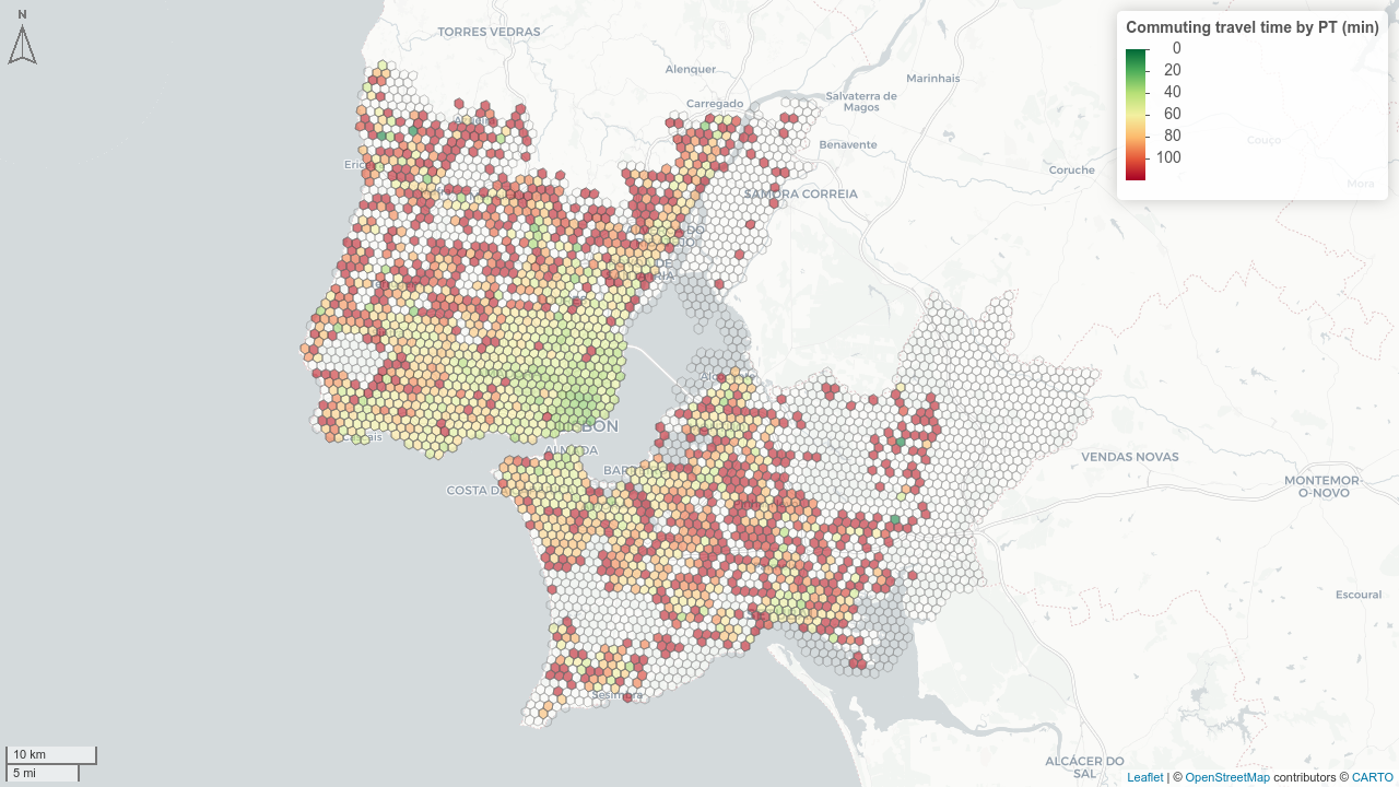
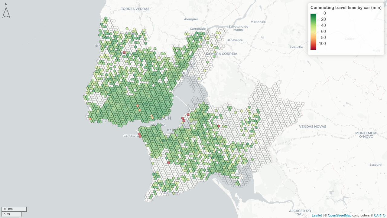
6.1 Commuting travel times

Script: 04_mobility_commuting.R

Using the jittered IMOB OD pairs (for commuting) and the travel time matrices, average commuting travel times are computed for each geographical unit and mode, weighted by number of trips (example at Figure 6.2). Trips with no feasible route within the constraints are assigned the maximum travel time (120 min) and counted separately as “not accomplishable” trips (PNA — Percentagem Não Alcançáveis).

flowchart TB
    TTM["Travel Time Matrix<br/>(all modes)"] --> Match
    ODs["Jittered OD pairs<br/>(IMOB 2017 commuting)"] --> Match
    Grid["H3 Grid"] --> Match
    
    subgraph Match["Spatial Assignment & Matching"]
        direction TB
        JoinGrid["Assign each OD<br/>to origin grid cell"] --> Lookup["Look up travel time<br/>for each OD pair<br/>in TTM"]
        Lookup --> Fill["Fill missing:<br/>max_duration = 120 min<br/>(NAs = not accomplishable)"]
    end
    
    Match --> AggMode["Aggregate by<br/>geographic unit × mode"]
    AggMode --> Output["avg_tt_{mode}<br/>trips, trips_na_{mode}<br/>PNA_{mode}"]

Figure 6.1: Commuting travel time computation

Public transport, up to 2 transfers

Car

Figure 6.2: Commuting travel time at grid level

6.2 Number of PT transfers

Script: 04_mobility_commuting.R

For each commuting OD pair, the minimum number of transfers required for each PTransit route (for 0, 1, 2, and 3 transfers) is assigned to each OD pair, and population-weighted mean transfers are computed per geographical unit. The result is the average minimum number of transfers to commute to work, using PTransit (Figure 6.3).

Figure 6.3: Average number of minimum transfers required for commuting with Public Transport

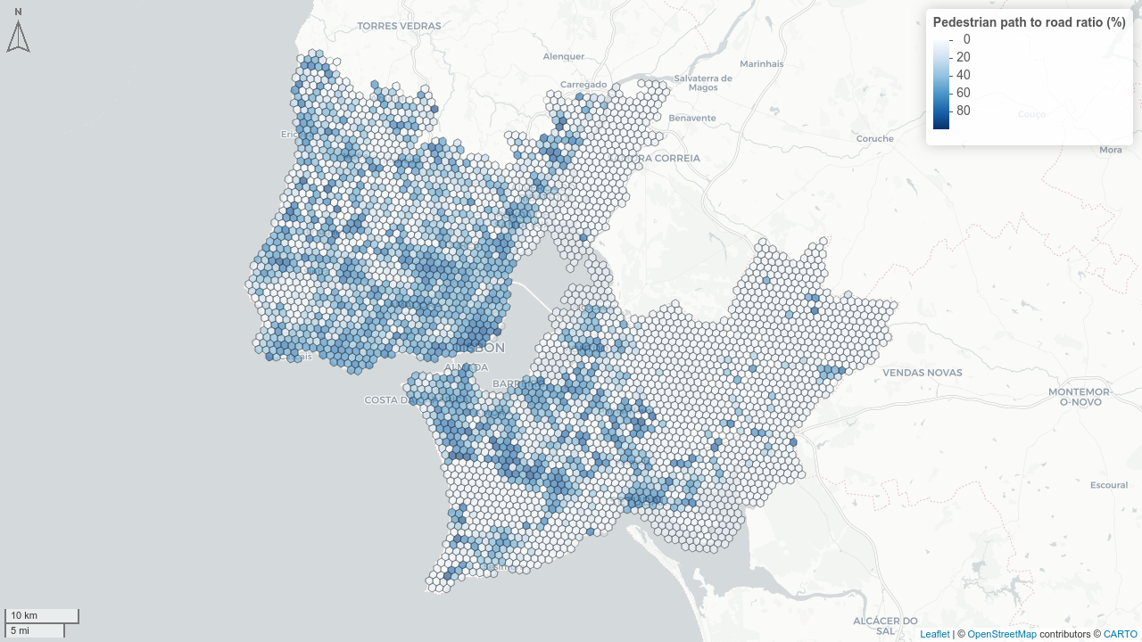
6.3 Walking and Cycling infrastructure ratio

Script: 04_mobility.R

6.3.1 Walking infrastructure ratio

The pedestrian infrastructure (Figure 6.4) ratio is the proportion of road length that includes pedestrian infrastructure, computed using OSM data:

\[R_{ped} = \frac{\text{pedestrian path length}}{\text{road length}}\]

Road classification uses highway tags: motorway, trunk, primary, secondary, tertiary, unclassified, residential, living_street, plus link variants.

Pedestrian infrastructure uses tags: highway = footway | pedestrian | steps | residential and footway = sidewalk | crossing | path | platform | corridor | alley | track, and sidewalk = both | left | right.

Figure 6.4: Walking infrastructure ratio at grid level

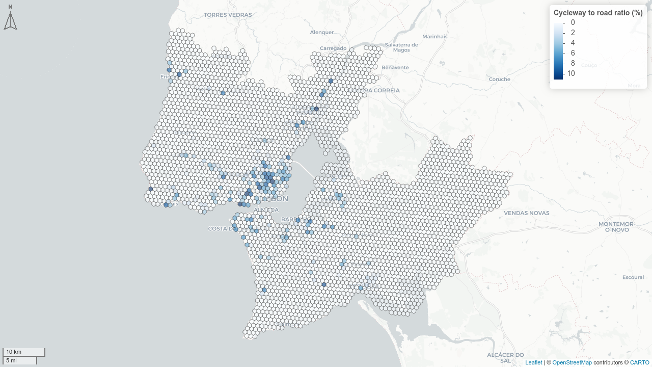
6.3.2 Cycling infrastructure ratio and type

Script: 04_mobility_bike_infrastructure.R

The cycling infrastructure ratio is computed analogously to the pedestrian ratio by comparing cycleway length to total road length. Infrastructure data is extracted from OpenStreetMap and classified according to its type and level of segregation:

• Cycle track or lane: Segregated or light-separated tracks exclusive for cycling (Ciclovia segregada).
  • highway = cycleway
  • highway = path & bicycle = designated
  • segregated = yes | no
  • cycleway tags containing: separate, buffered_lane, segregated, lane, or track.
• Advisory lane: Marked cycle lanes shared with motor vehicles, such as sharrows or advisory lanes (Via partilhada com veículos motorizados / zonas 30).
  • cycleway tags containing: shared_lane.
• Protected Active: Infrastructure shared with pedestrians but protected from motor vehicles (Via partilhada com peões).
  • highway = pedestrian & bicycle = designated.
  • Refinement of highway = path | footway | pedestrian when foot access is explicitly allowed on cycling paths without physical segregation.

The primary indicators are:

Cycling infrastructure ratio (Figure 6.5): \[R_{cyc} = \frac{\text{total cycleway length}}{\text{road length}}\]

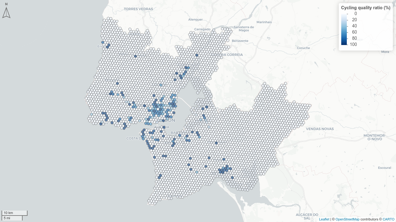
Cycling quality ratio (Figure 6.6): \[R_{cyc,q} = \frac{\text{segregated cycleway length}}{\text{total cycleway length}}\]

Where “segregated cycleway length” corresponds to the Cycle track or lane category.

Figure 6.5: Cycling infrastructure ratio at grid level

Figure 6.6: Cycling quality ratio at grid level

6.4 PT stop coverage

Scripts: 04_isochrones_PTstops.R, 04_mobility_transit_population.R
Package: r5r (Pereira et al. 2021)

Population coverage by public transport is estimated using walking isochrones around PT stops, differentiated by transport mode and their typical service area. Isochrones are computed with r5r::isochrone() using the WALK mode and the AML street network.

6.4.1 Isochrone estimation by PT mode

Three mode groups are defined based on stop type (identified from GTFS stop_id prefixes) and their standard catchment areas:

Table 6.1: PT mode groups and walking catchment thresholds

Mode group	Operators	Walking threshold	Rationale
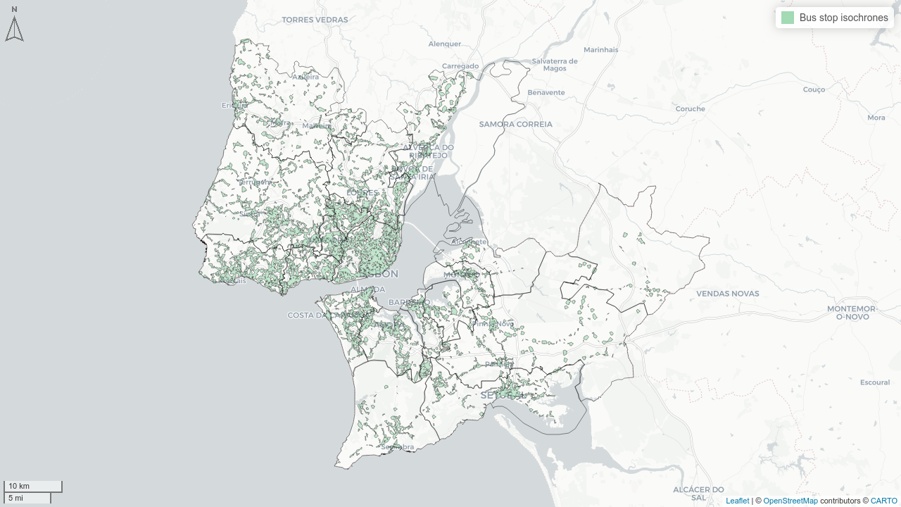
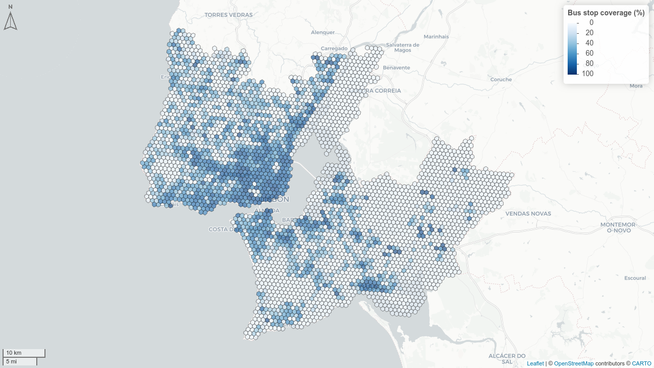
Bus	Carris, MobiCascais, Transportes Colectivos Barreiro	5 minutes	High-density stop network; short acceptable walk
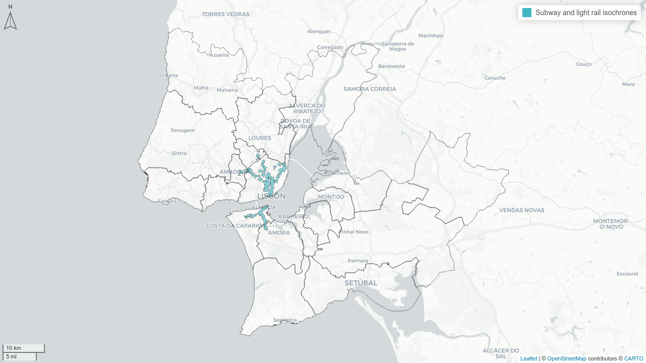
Subway & light rail	Metro de Lisboa, MTS	10 minutes	Fewer stops, higher service quality
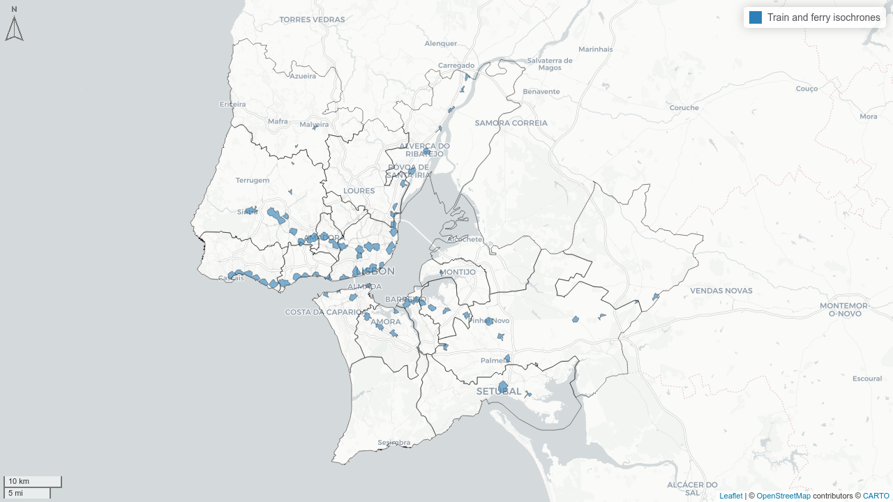
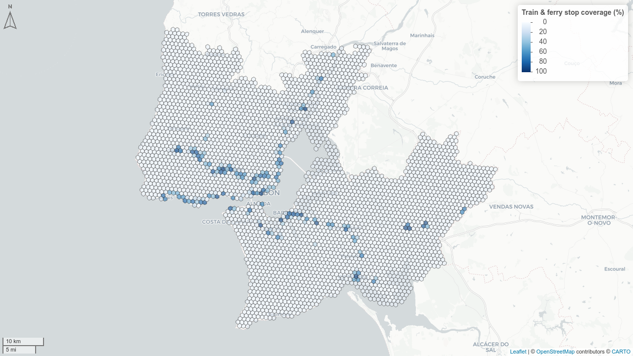
Train & ferry	CP, Fertagus, Transtejo, Soflusa	15 minutes	Sparse network; users accept longer walks

Bus stops are first consolidated by merging stops within 30 m of each other into a single representative centroid (using a 15 m buffer union), reducing the dataset from ~16 000 to ~10 700 origins before routing. Isochrones are computed in batches and dissolved into a single polygon per mode group. Stops that could not be routed are replaced with 300 m Euclidean buffers.

A union isochrone is computed from all three layers (Figure 6.7) to estimate coverage by any PT mode, avoiding double-counting of population in overlapping catchment areas.

Bus isochrones

Subway & light rail isochrones

Train & ferry isochrones

Figure 6.7

6.4.2 Population estimation (dasymetric method)

All methods share the same COS residential building polygons as the spatial proxy for where population lives, weighted by residential density class:

Table 6.2: Population and building density weights for COS land use classes

COS class	Weight
Contínuas predominantemente verticais	3.0
Contínuas predominantemente horizontais	1.0
Descontínuas	0.6
Descontínuas esparsas	0.3

Different aggregation strategies are used at each scale, due to the geometric relationship between spatial units:

6.4.2.1 Grid level (H3 r8)

Because H3 hex boundaries do not align with COS or BGRI polygon boundaries, a fragment-centroid approach would assign a building fragment’s entire population to one hex even when the fragment straddles two. To avoid this mismatch, the grid-level method computes the fraction of each hex’s weighted COS building area that falls inside the isochrone:

\[f_i = \frac{\sum_{k} A_{k \cap \text{iso} \cap \text{hex}_i} \times w_k}{\sum_{k} A_{k \cap \text{hex}_i} \times w_k}\]

where \(k\) indexes COS polygons and \(w_k\) is the density weight. Population served is then:

\[P_i = \text{pop}_i \times f_i\]

where \(\text{pop}_i\) is the hex population from the dasymetric grid (grid_with_cos).

6.4.2.2 Freguesia and município levels

BGRI census blocks nest perfectly within administrative boundaries. The method therefore uses building fragments — intersections of COS polygons with BGRI blocks — and apportions each BGRI’s population by the fraction of its weighted building area that falls inside the isochrone:

\[P_{iso} = \sum_{\text{fragments}} N_{\text{BGRI}} \times \frac{A_{frag,iso} \times w_{frag}}{\sum_{\text{BGRI}} A_{frag} \times w_{frag}}\]

The centroid of each fragment is used to assign it to the administrative unit, and fragments go directly to administrative boundaries — not via the grid — to avoid misalignment from hexes that only partially overlap them. Total population for percentage calculations is derived from the same building fragment method, not from raw BGRI totals, ensuring a consistent denominator.

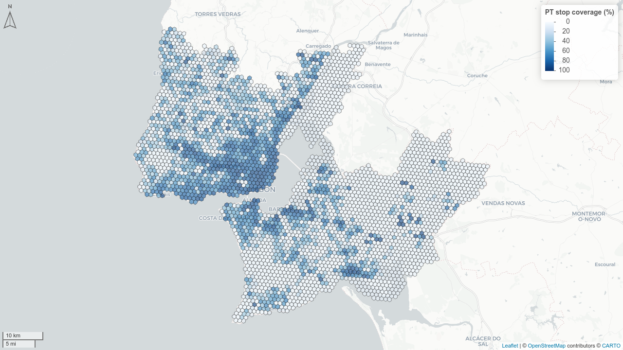
Metrics produced per mode group and scale:

• pop_pt_{mode} — population within walking distance of each mode (or all modes)
• pct_pt_{mode} — percentage of population within walking distance of each mode (or all modes) (Figure 6.8)

All PT modes

Bus

Subway & light rail

Train & ferry

Figure 6.8: Percentage of population within walking distance of each mode (or all modes)

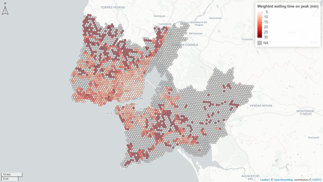
6.5 PT headways and waiting times

Script: 04_mobility_transit.R
Package: tidytransit (Poletti et al. 2026)

Stop-level service frequencies are computed with tidytransit::get_stop_frequency() for four time windows:

Table 6.3: PT service frequency periods

Period	Date	Time window
Weekday peak	Wed 04/02/2026	08:00–09:00
Weekday full day	Wed 04/02/2026	00:00–48:00
Weekday night	Wed 04/02/2026	22:00–23:00
Weekend	Sun 08/02/2026	10:00–11:00

A 500 m buffer per stop is used to allocate stops to census population centroids. Results are aggregated to parishes and municipalities as population-weighted mean headway and waiting time (example in Figure 6.9).

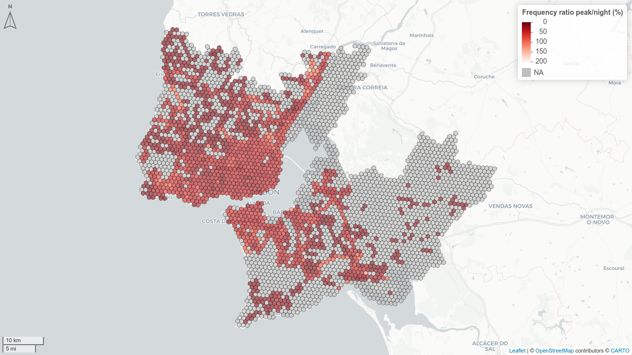
Additionally, frequency reduction factors are computed to characterise night and weekend service reduction (example in Figure 6.10).

Figure 6.9: Average waiting time at peak

Figure 6.10: Frequency ratio peak/night

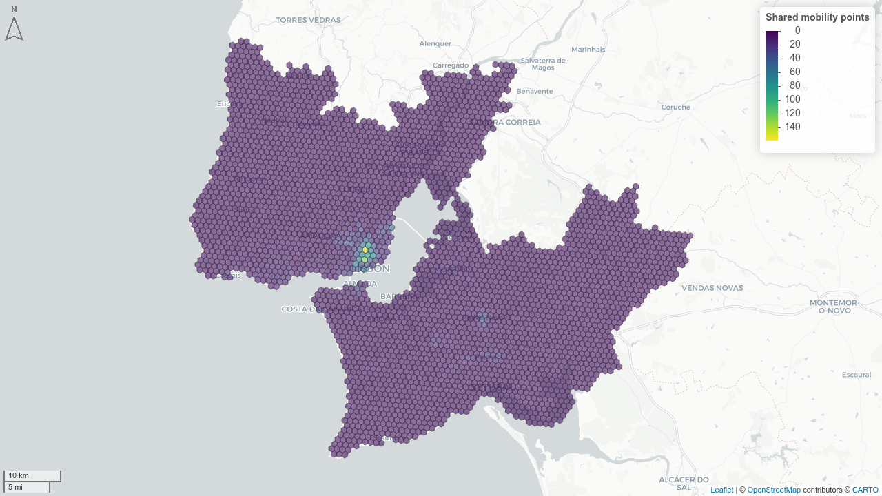
6.6 Shared mobility

Script: 04_mobility.R
Source: TML PMUS (Shared mobility dock locations) (TML and Way2Go 2025)

The number of shared mobility points (physical and virtual docks) is counted per parish and per grid cell (Figure 6.11).

Figure 6.11: Shared mobility points

Pereira, Rafael H. M., Marcus Saraiva, Daniel Herszenhut, Carlos K. V. Braga, and Matthew Wigginton Conway. 2021. “R5r: Rapid Realistic Routing on Multimodal Transport Networks with R5 in R.” Findings. https://doi.org/10.32866/001c.21262.

Poletti, Flavio, Daniel Herszenhut, Mark Padgham, Tom Buckley, Danton Noriega-Goodwin, Angela Li, Elaine McVey, et al. 2026. “Tidytransit: Read, Validate, Analyze, and Map GTFS Feeds.” https://cran.r-project.org/web/packages/tidytransit/index.html.

TML, Transportes Metropolitanos de Lisboa, and Consultores Associados Lda. Way2Go. 2025. “PMMUS – Plano Metropolitano de Mobilidade Urbana Sustentável Da amL.” https://pmmus.tmlmobilidade.pt/.