[[10]{.chapter-number}  [Index Computation — IMPT Calculator]{.chapter-title}]{#sec-calculator .quarto-section-identifier}

10 Index Computation — IMPT Calculator

Script: 05_IMPTcalculator.R
Package: FactoMineR (PCA) (Husson et al. 2026)

flowchart TB
    %% Nodes
    AccIn["Accessibility indicators"]
    MobIn["Mobility indicators"]
    AffIn["Affordability indicators<br>(two fare scenarios)"]
    SafIn["Safety indicators"]
    
    Ben["Benefit indicators<br>min→1, max→100<br>normalize_benefit()"]
    Cost["Cost indicators<br>min→100, max→1<br>normalize_cost()"]
    
    Run["FactoMineR::PCA()<br>extract PC1 scores"]
    Scale["Rescale PC1 to [1,100]<br>scale_0_100()"]
    Direction["Validate direction:<br>check correlation with<br>top indicator"]
    
    Geom["Geometric mean<br>(Acc * Mob * Aff * Safety)^0.25"]
    EntrW["Entropy-weighted mean<br>compute_entropy_weights()"]
    Simple["Simple arithmetic mean<br>(Acc + Mob + Aff + Safety) / 4"]
    
    SpatialAgg["Population weighted<br>aggregation"]
    Out["Final IMPT scores:<br>freiguesia, municipality, grid<br>× global and per mode"]

    %% Connections
    subgraph Inputs["Input Dimension Tables (by parish)"]
        direction TB
        AccIn ~~~ MobIn ~~~ AffIn ~~~ SafIn
    end
    
    Inputs --> Normalise
    
    subgraph Normalise["Normalisation to [1,100]"]
        direction LR
        Ben ~~~ Cost
    end
    
    Normalise --> PCA
    
    subgraph PCA["PCA per dimension (global & per mode)"]
        direction LR
        Run ~~~ Scale ~~~ Direction
    end
    
    PCA --> Composite
    
    subgraph Composite["Composite IMPT Score"]
        direction LR
        Geom ~~~ EntrW ~~~ Simple
    end
    
    Composite --> SpatialAgg
    SpatialAgg --> Out

    %% Subgraph styling
    style Inputs fill:#f8f9fa,stroke:#adb5bd,stroke-width:1px,color:#212529
    style Normalise fill:#f8f9fa,stroke:#adb5bd,stroke-width:1px,color:#212529
    style PCA fill:#f8f9fa,stroke:#adb5bd,stroke-width:1px,color:#212529
    style Composite fill:#f8f9fa,stroke:#adb5bd,stroke-width:1px,color:#212529

Figure 10.1: IMPT index computation pipeline

10.1 Normalisation

All indicators are normalised to the range [1, 100] using min-max scaling:

Benefit indicators (higher raw value → better): \[X_{norm} = 1 + \frac{X - X_{min}}{X_{max} - X_{min}} \times 99\]

Cost indicators (lower raw value → better): \[X_{norm} = 1 + \frac{X_{max} - X}{X_{max} - X_{min}} \times 99\]

Accessibility metrics (access_*) are benefit indicators.
Mobility cost metrics (mobility_cost_*), PT waiting times, all affordability indicators, and all safety indicators are cost indicators.

Missing values in accessibility indicators (arising from infeasible PT routes) are imputed with the mean of the respective variable prior to PCA.

10.2 PCA-Based Dimension Scores

For each dimension (Accessibility, Mobility, Safety) and at the global (all-mode) and per-mode levels, a PCA is run using FactoMineR::PCA() at parish level.

The first principal component (PC1) score is used as the dimension index, after rescaling to [1, 100]. PC1 captures the dominant axis of variation among the normalised indicators.

For Affordability, PCA is not applied (too few indicators); instead, the normalised composite h_transp_inc_comp (housing + transport cost as share of income, modal-share weighted) is used directly as the Affordability Index.

For Safety per mode, an equal-weight average of the severity index (per mode) and total vehicles involved (per mode) is used instead of PCA.

For Mobility - Car PCA is not applied (too few indicators); instead, we assumed an equal-weight average of the normalized composite mobility_commuting_avg_tt_car and road_length.

10.3 Composite IMPT Scores

Three aggregation methods are computed for the global IMPT and each per-mode IMPT:

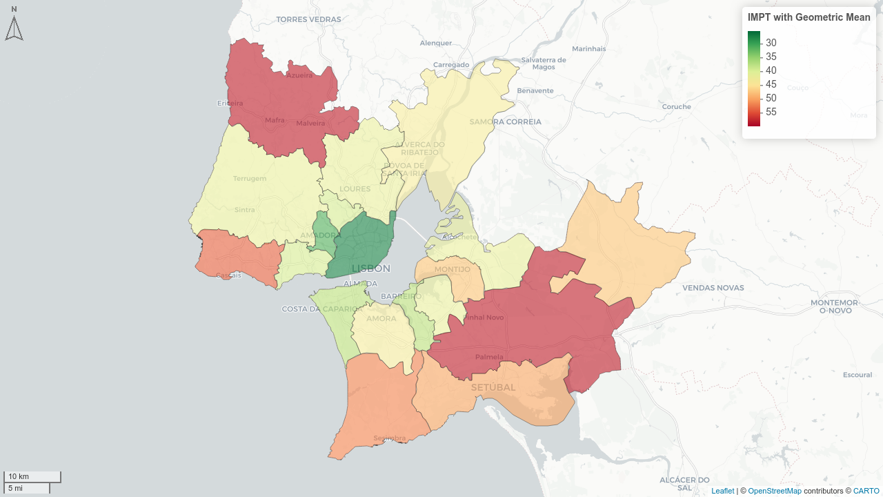
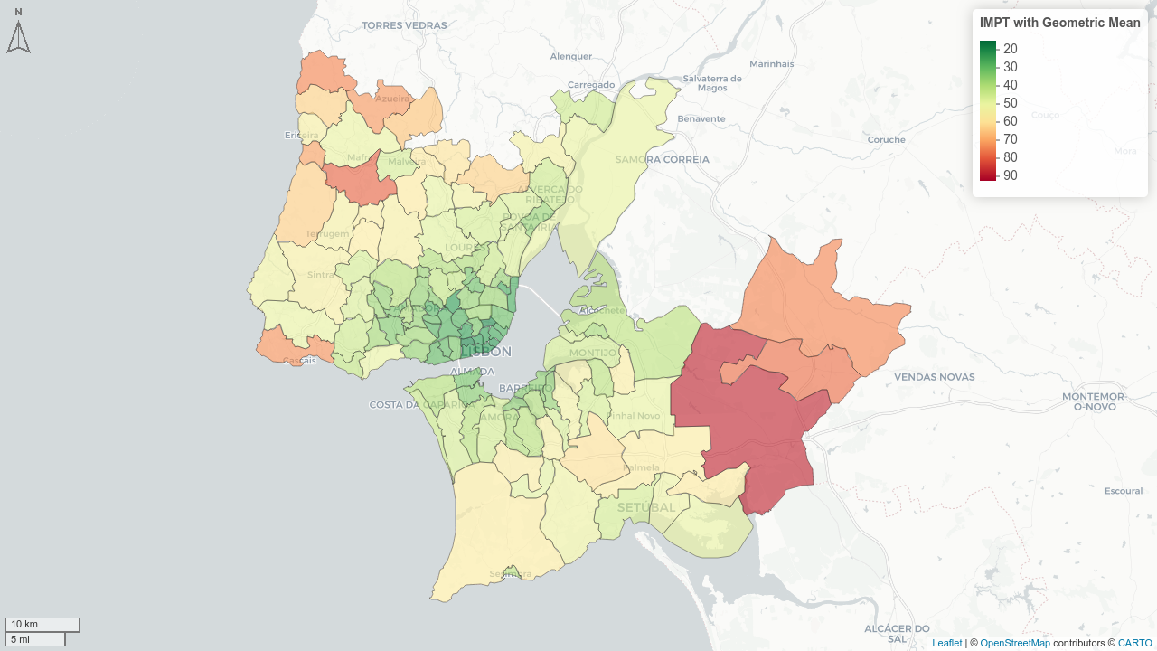
Geometric mean (equal weights, Figure 10.2 (a)): \[IMPT_{geom} = \left(\prod_{d} (S_d + 1)\right)^{1/n} - 1\]

Partially compensatory: penalizes dimensions with very low values non-linearly. Highlights the most critical situations, where at least one dimension is severely deficient.

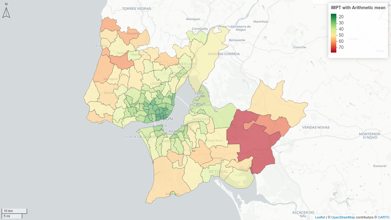
Arithmetic mean (equal weights, Figure 10.2 (b)): \[IMPT_{avg} = \frac{1}{n} \sum_d S_d\]

Compensatory: high vulnerability in one dimension can be offset by good performance in others. Suitable for setting aggregate policy targets and communicating to non-specialist audiences.

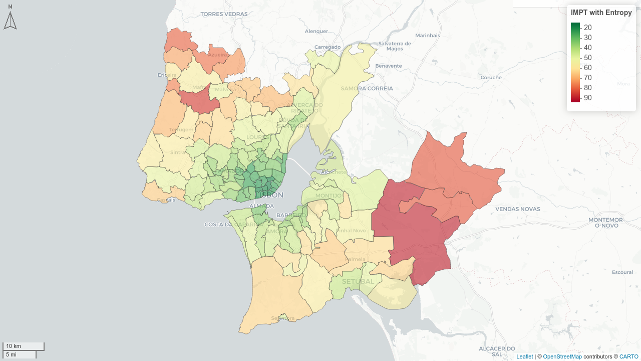
Entropy-weighted geometric mean (Figure 10.2 (c)): \[IMPT_{entropy} = \prod_d (S_d + 1)^{w_d} - 1\]

where weights \(w_d\) are derived from the entropy weighting method:

Weights are determined by the empirical dispersion of the dimensions across parishes: the dimension that varies most among territories receives greater weight. Maximises territorial contrast and is useful for competitive prioritisation of interventions.

\[w_d = \frac{d_d}{\sum_j d_j}, \quad d_d = 1 - e_d, \quad e_d = -k \sum_i p_{id} \ln(p_{id})\]

with \(k = 1/\ln(n)\) and \(p_{id}\) being the proportion of the dimension score for area \(i\).

10.4 Spatial Aggregation

Once scores are computed at parish level, they are aggregated to higher and lower levels:

Municipality level: population-weighted mean of parish scores (example in Figure 10.3 (a)).
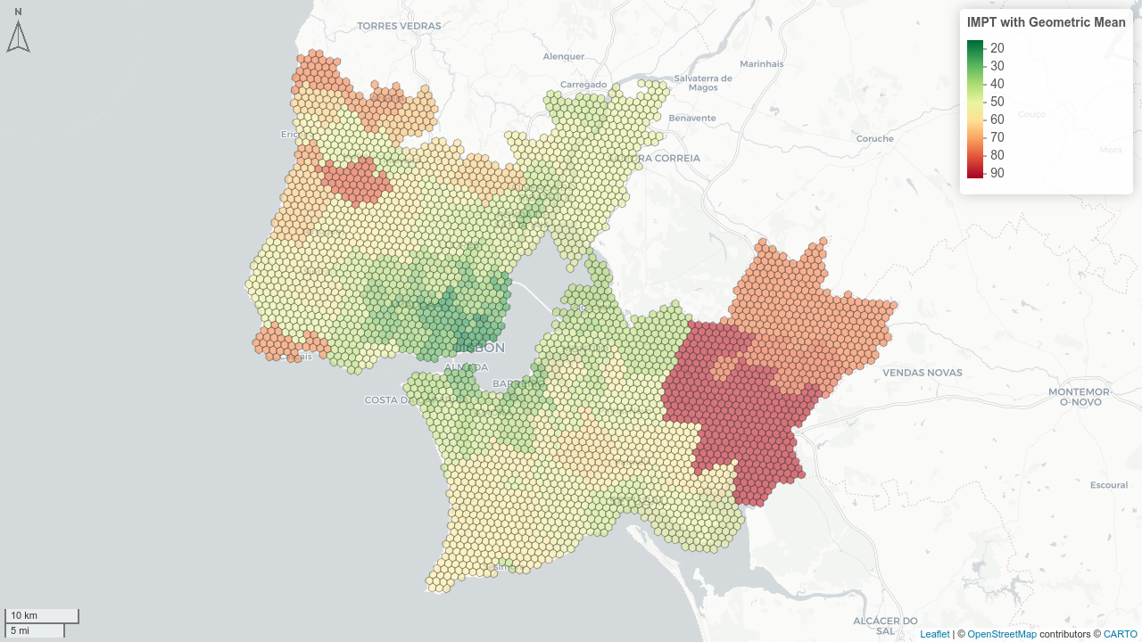
Grid level: parishes are assigned to grid cells via the grid_nuts.csv cross-reference table; scores are assigned from the host parish (no further averaging at this stage) (example in Figure 10.3 (b)).