flowchart LR
    AML["AML boundary<br/>CAOP 2024"] --> H3["h3jsr::polygon_to_cells<br/>Resolution 8"]
    H3 --> Cells["3,686 hexagons<br/>531m edge, 0.74 km2 avg"]
    Cells --> C["Grid centroids<br/>for routing"]
    Cells --> G["Grid index table<br/>mapping levels"]
4 Data Preparation
Note
This phase corresponds to scripts 00b_*, 01_* and 02_* in the pipeline.
4.1 Study Area
00b_data_load.R sets up globally-used variables (study area boundaries, grid, ids correspondence between levels, etc.) that are reused across scripts.
To run for different study areas, this script must be updated to reflect the desired boundaries.
4.2 Administrative Boundaries
Source: CAOP 2024.1 (DGT 2024)
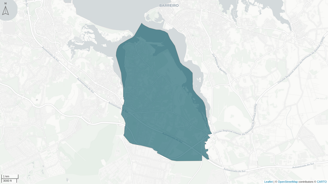
The full continental Portugal polygon file is filtered to the Grande Lisboa and Península de Setúbal NUTS-II sub-regions. For the municipality of Lisboa, parish boundaries with the Tagus estuary are replaced by clipped geometries (FREGUESIASgeo.gpkg - using CAOP 2016 parish limits) to remove the water area in Lisbon municipality (Figure 4.1).
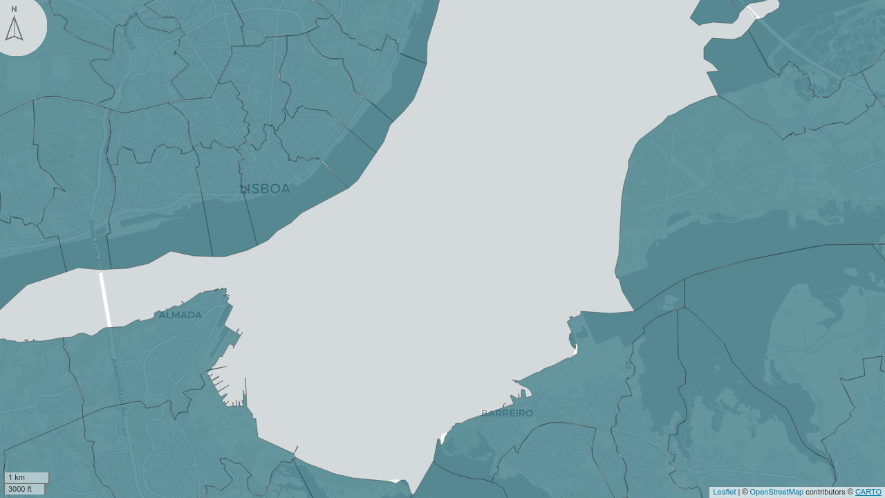
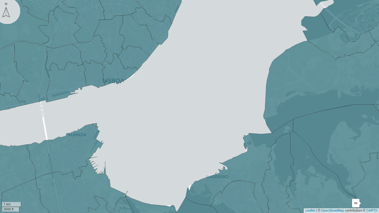
For parishes with multiple polygon features (due to small islands), only the polygon with the largest area is retained.
4.2.1 Conversion of 2016 to 2024 Parish Codes
The Census 2021 and IMOB 2017 travel survey use 2016 parish codes (DICOFRE). Several parishes were split between 2016 and 2024. A manual conversion table was created after inspecting the differences:
| Old DICOFRE (2016) | New DICOFRE(s) (2024) |
|---|---|
| 151007 | 151008, 151009, 151010 |
| 111127 | 111134, 111135 |
| 111123 | 111129, 111131, 111132 |
| 111126 | 111130, 111133 |
Trips associated with split parishes were redistributed proportionally to the area of the new parishes. Conservation of total trip counts was validated using assertthat.

4.3 H3 Hexagonal Grid
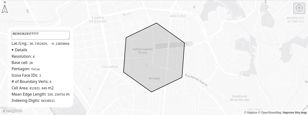
The H3 hexagonal grid (Uber Technologies 2018) is generated at Resolution 8 using the h3jsr package (O’Brien 2023). Resolution 8 (example at Figure 4.4) provides a spatial unit with an average edge length of ~531 m and average area of ~0.74 km², which offers a good balance between spatial detail and computational tractability for routing-based accessibility measures.
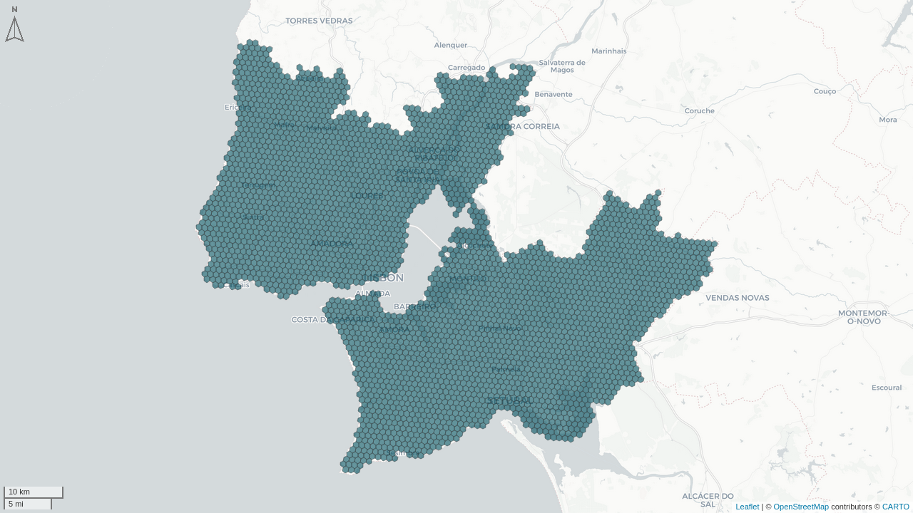
The H3 grid covers the AML with 3,686 active hexagons (those intersecting the administrative boundaries, see Figure 4.5). At the limits, if a hexagon covers less than 50% of the administrative area, it is excluded from the analysis. Each hexagon is assigned to a parish and municipality via a cross-reference table (grid_nuts.csv).
4.4 Census Data Processing
Source: INE Census 2021, BGRI 2021 at the base statistical unit level (INE 2021a), NUTS-3 Área Metropolitana de Lisboa (code 170).
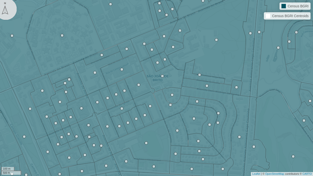
Census BGRI polygons are converted to centroids (Figure 4.6). The following variables are extracted:
| Variable | INE field | Description |
|---|---|---|
population |
N_INDIVIDUOS |
Total residents |
households |
N_NUCLEOS_FAMILIARES |
Total households |
youth |
N_INDIVIDUOS_0_14 |
Residents aged 0–14 |
adults |
N_INDIVIDUOS_15_24 + N_INDIVIDUOS_25_64 |
Residents aged 15–64 |
elderly |
N_INDIVIDUOS_65_OU_MAIS |
Residents aged 65+ |
women |
N_INDIVIDUOS_M |
Female residents |
buildings |
N_EDIFICIOS_CLASSICOS |
Classic buildings |
buildings_pre1945 |
N_EDIFICIOS_CONSTR_ANTES_1945 |
Buildings built before 1945 |
For parish- and municipality-level aggregation, census data from 2016-era parishes are redistributed to 2024 parishes using the area-weighted conversion table described in Section 4.2.1.
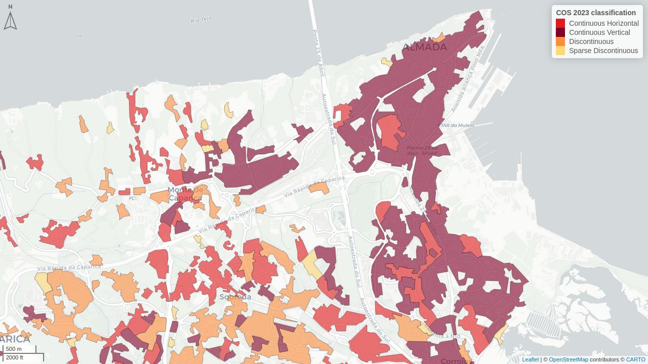
4.5 Dasymetric Grid Population Redistribution (COS 2023)
Source: COS 2023 v1 (DGT 2023), residential land use classes
To achieve a more accurate population distribution within the H3 grid, a dasymetric mapping approach is applied using the Carta de Ocupação do Solo (COS) 2023 (example in Figure 4.7). This is a relevant method, in particular when dealing with BGRI polygons that cover large areas, across multiple hexagons cells - preventing that one single hexagon is assigned the entire population of the BGRI polygon with it’s centroid.
Residential areas are extracted with the following classes and assigned weighting factors:
| COS 2023 classification | Weight |
|---|---|
| Contínuas predominantemente verticais | 3.0 |
| Contínuas predominantemente horizontais | 1.0 |
| Descontínuas | 0.6 |
| Descontínuas esparsas | 0.3 |
The procedure (02_census_grid_with_cos.R):
- Census BGRI polygons are intersected with COS residential patches and H3 grid cells.
- For each BGRI fragment, a weighted score is computed as
fragment_area × weight. - Each BGRI’s population is distributed proportionally to the weighted score of each fragment.
- Results are summed per H3 cell.
This recovers approximately 99.4% of the total AML population (2,854,660 vs. 2,870,208 in the census), a significant improvement over simple centroid assignment.
Important
The land use and census data from the dasymetric method is only used at the grid level for the calculation of fine-grain indicators. For the other levels, the Census 2021 BGRI data is used directly.
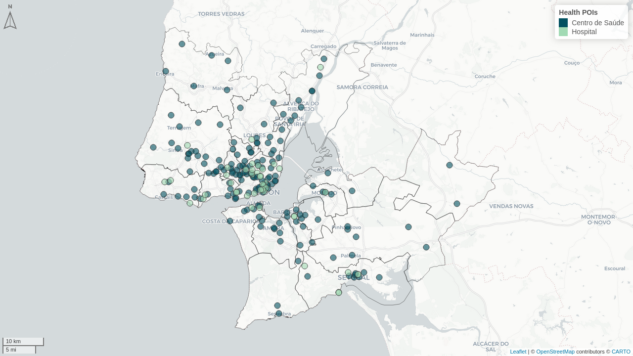
4.6 Points of Interest (POIs)
POIs are collected from three sources: OpenStreetMap (OpenStreetMap 2026), Carris Metropolitana open datasets (Carris Metropolitana 2026), and GTFS feeds. The following categories are used:
| Category | Identifier | Source | Filter / Description |
|---|---|---|---|
| Healthcare (all) | health | CM | All health centres |
| Hospitals | health_hospital | CM | name contains 'Hospital' or 'Centro de Medicina' |
| Primary care centres | health_primary | CM | name contains 'Centro de Saúde' |
| Supermarkets/grocery | groceries | OSM | type %in% c('supermarket','convenience') |
| Green spaces | greenspaces | OSM | group == 'leisure' & type %in% c('park','garden') |
| Recreation | recreation | OSM | type %in% c('library','theatre','cinema','restaurant','cafe','bar','pub','pitch','fitness_station','swimming_pool','sports_centre','fitness_center') |
| Schools (all) | schools | CM | All school types |
| Primary schools | schools_primary | CM | pre_school==1 | basic_1==1 | basic_2==1 | basic_3==1 |
| Transit stops (all) | transit | GTFS (all operators) | All stops from all operators |
| Transit stops (bus) | transit_bus | GTFS (Carris, CM, TCB, Cascais próxima) | Bus operators only |
| Transit stops (mass transit) | transit_mass | GTFS (CP, Fertagus, Metro, MTS, TTSL) | Rail, metro, ferry operators |
| Jobs | jobs | IMOB 2018 | Jittered OD destinations (see #sec-jittering) |
4.7 Travel Survey Data and OD Jittering
Source: IMOB 2017/18 (INE 2018)
The IMOB survey served as base to produce the OD matrix at parish level with modal split (walk, bike, car, public transit, other), available at biclaR project.
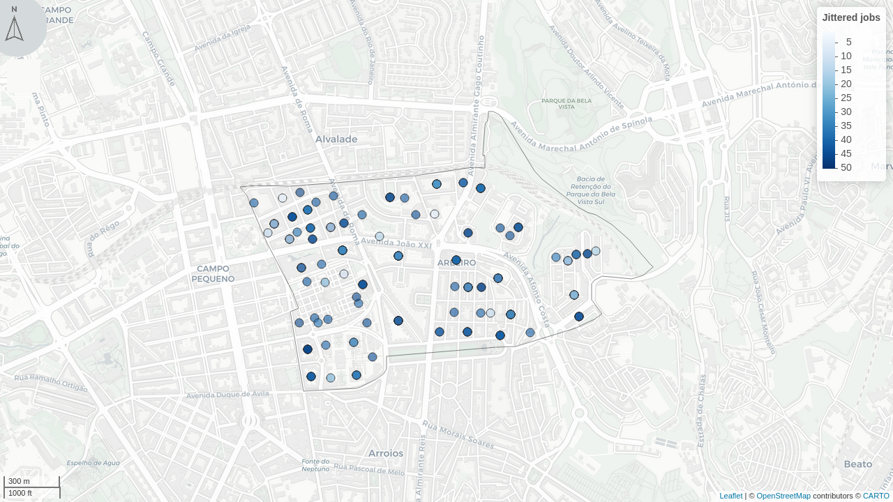
4.7.1 Jobs as a proxy
Since high-resolution employment data was not available (or open) for the AML during the report development, employment locations were proxied using the jittered destinations of trips from the IMOB 2017 travel survey. Specifically, trips with the purpose “Ir para o trabalho” (Commute to work) and “Tratar de assuntos profissionais” (Work-related business) were extracted, and their jittered destination points were used as POIs representing the spatial distribution of jobs.
Since accessibility and cost computations require disaggregated spatial locations, jittering is applied to generate point-level OD pairs.
NoteAlternative data source: Ministério do Trabalho
TML has reported to use Ministério do Trabalho dataset on jobs for the Metropolitan Sustainable Urban Mobility Plan. However, they only kept them aggregated at the grid level, using a custom grid that is not compatible with the H3 grid used in this project. For future versions of IMPT, a request can be made to Ministério do Trabalho for the original data.
4.7.2 Jittering Algorithm
Jittering is performed using the odjitter R package (Carlino and Lovelace 2022), following the approach described in Lovelace, Félix, and Carlino (2022).
The algorithm disaggregates parish-level trip counts into point-to-point flows. The following layers and weights are used:
- Origins: Randomly sampled points within residential buildings.
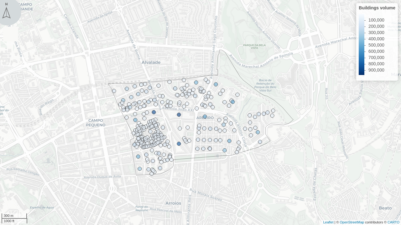
- Destinations: Sampled from a building layer (from
GDA), weighted by building volume (estimated asheight * footprint_m2). This ensures that areas with higher office and industrial density attract more jittered trips. - Threshold: A disaggregation threshold of 50 trips is applied, meaning any OD flow with more than 50 trips is split into multiple point-to-point pairs to provide higher spatial resolution.
- Deterministic Randomization: A fixed seed (
rng_seed = 42) is used to ensure the generated points are consistent across pipeline runs.
The process, illustrated in Figure 4.9, generates approximately 18,500 jittered OD pairs representing the daily commuting pattern in the AML. This is then expanded to the real number of trips using the PESOFIN weights.
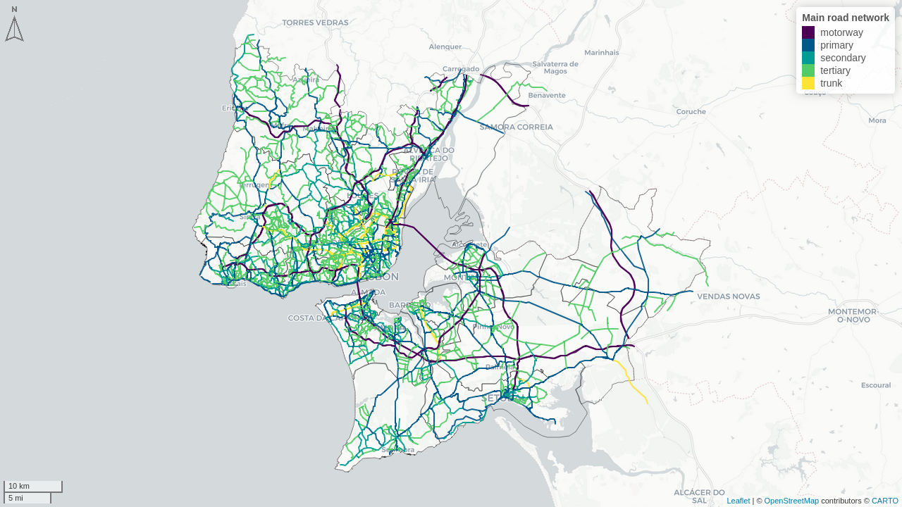
4.8 Road Network and DEM
Road network: Exported from HOT Export Tool (HOT 2026) in .pbf format for use with r5r (Pereira et al. 2021). Main network shown in Figure 4.10. The network includes all OSM road types and GTFS transit feeds.
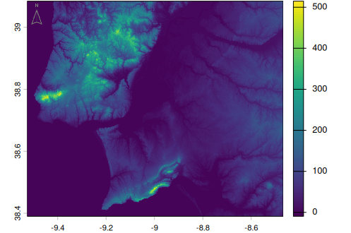
Elevation: Digital Elevation Model at 30 m resolution (Figure 4.11) downloaded from Copernicus ESA (EU 2026). Used to account for topographic effects on walking and cycling travel times via the Minetti metabolic-equivalent cost function.
The r5r network is built using r5r::build_network() with the elevation = "MINETTI" option.
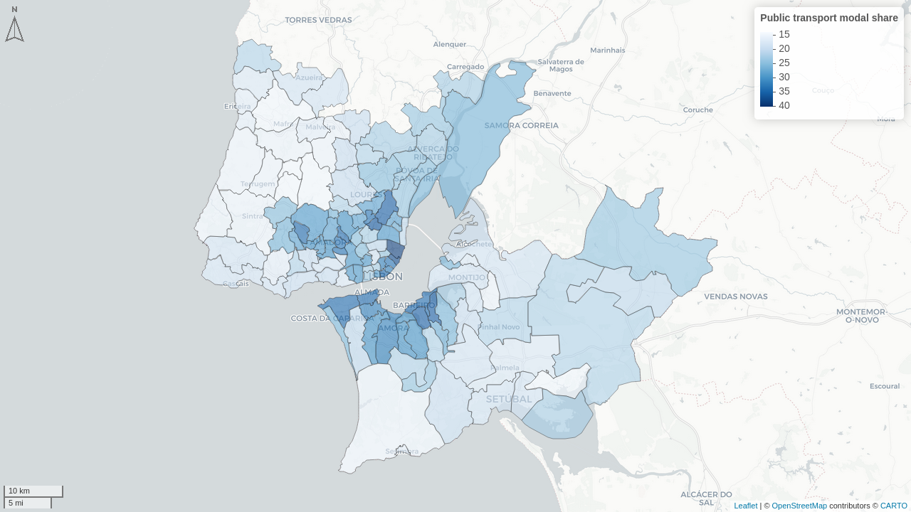
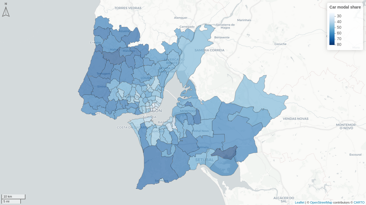
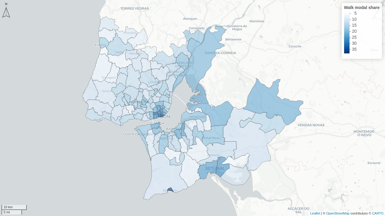
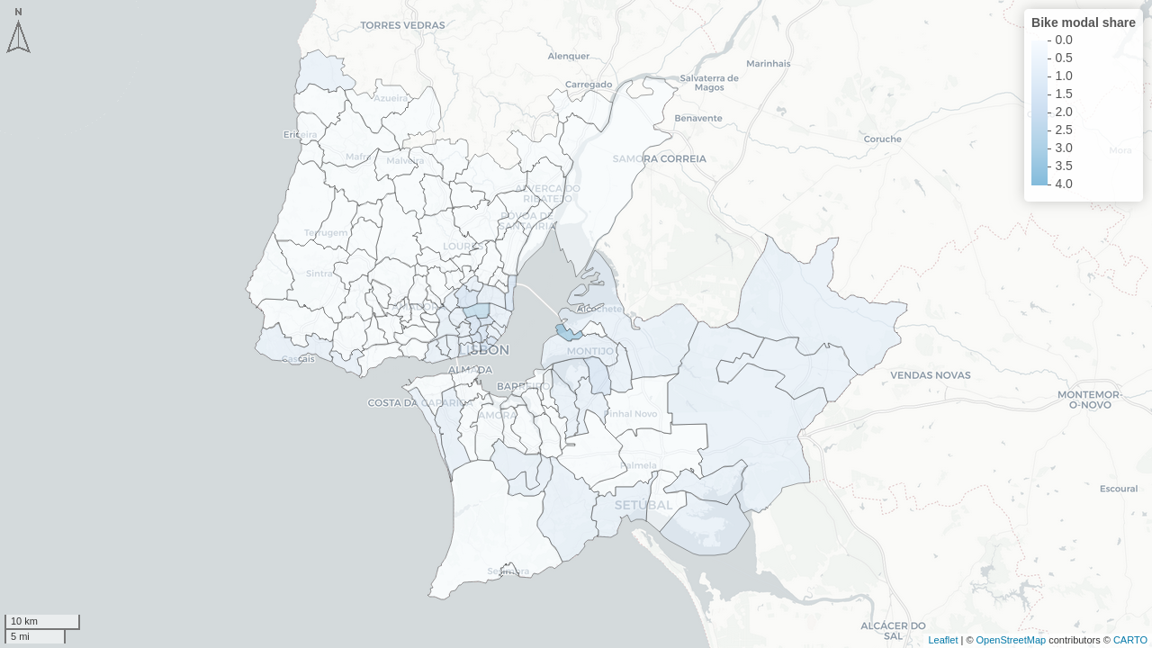
4.9 Modal Share from Census
Source: Census 2021 (INE 2021b)
Script 02_census_modalShare.R extracts and computes modal shares (private vehicle, public transport, active modes) at parish (Figure 4.12) and municipality level. These are used to compute modal-share-weighted affordability metrics (see Chapter 8).
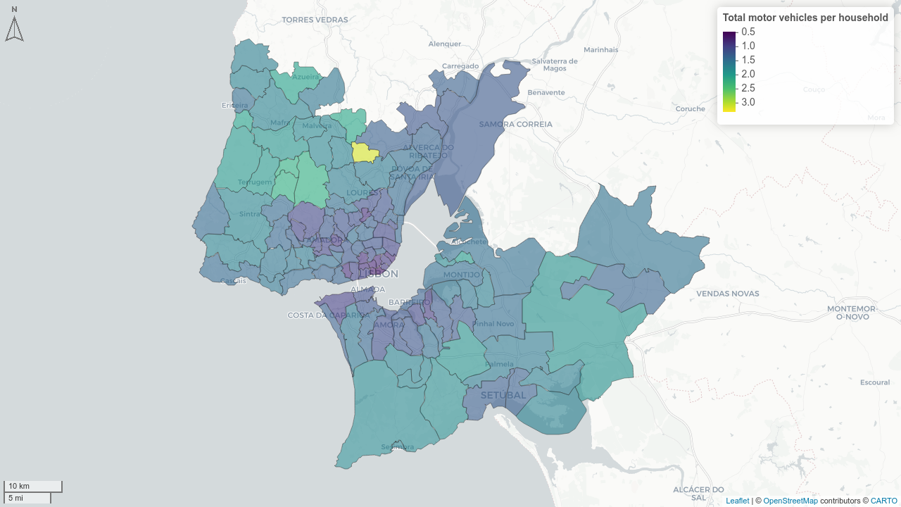
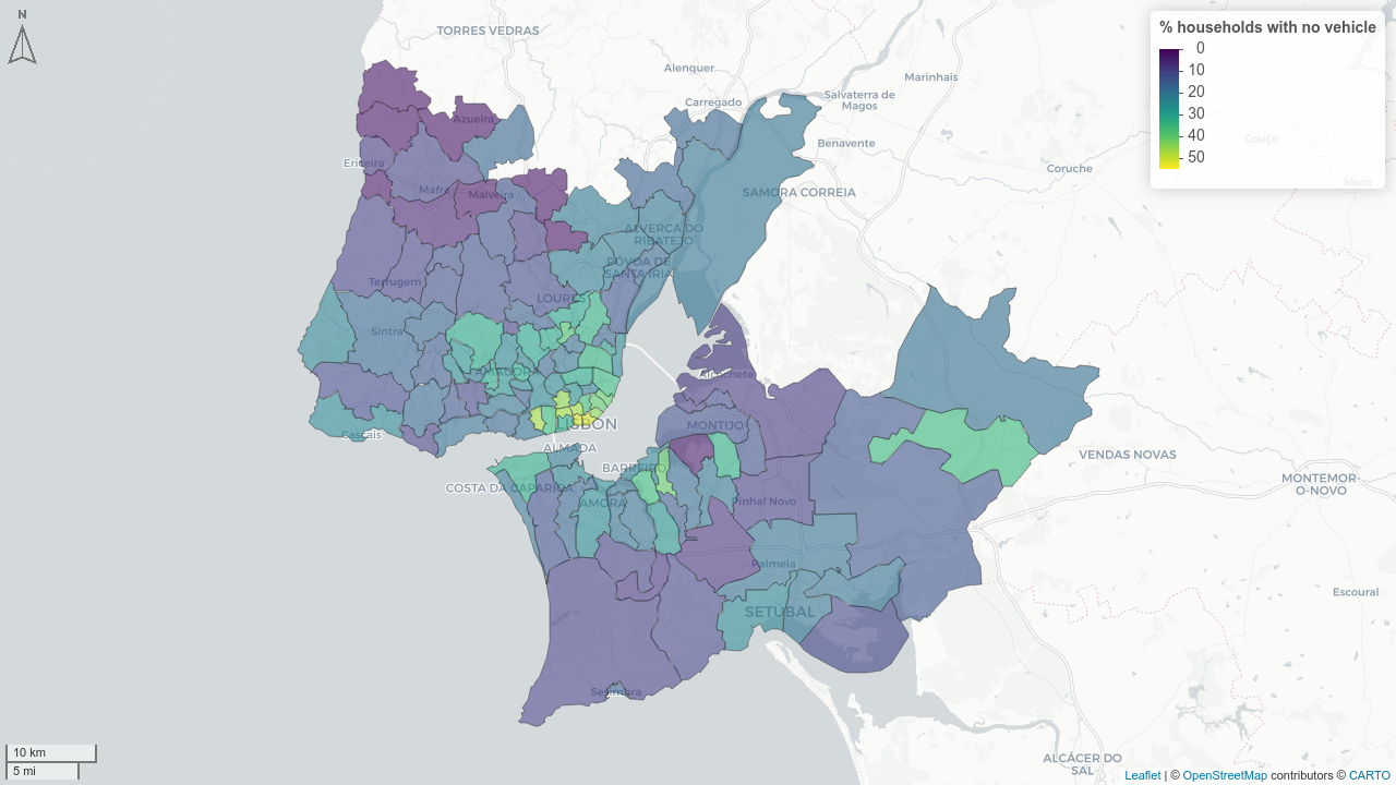
4.10 Vehicle Ownership
Source: IMOB 2017 data (INE 2018)
Vehicle ownership variables include average motorised vehicles per household (Figure 4.13) and percentage of households without a vehicle (Figure 4.14), aggregated at parish and municipality level. Calculations performed in 02_veh_ownership.R.