Code
library(dplyr)

SURVEY = read.csv("data/SURVEY.txt", sep = "\t") # tab delimiter
names(SURVEY)
[1] "ID" "AFF" "AGE" "SEX" "MODE" "lat" "lon" We will show how to estimate euclidean distances (as crown flights) using sf package, and the distances using a road network using r5r package (demonstrative).
Taking the survey respondents’ location, we will estimate the distance to the university (IST) using the sf package.
We will use a survey dataset with 200 observations, with the following variables: ID, Affiliation, Age, Sex, Transport Mode to IST, and latitude and longitude coordinates.
library(dplyr)
SURVEY = read.csv("data/SURVEY.txt", sep = "\t") # tab delimiter
names(SURVEY)[1] "ID" "AFF" "AGE" "SEX" "MODE" "lat" "lon" As we have the coordinates, we can convert this data frame to a spatial feature, as explained in the Introduction to spatial data section.
library(sf)

SURVEYgeo = st_as_sf(SURVEY, coords = c("lon", "lat"), crs = 4326) # convert to as sf dataUsing coordinates from Instituto Superior Técnico, we can directly create a simple feature and assign its crs.
UNIVERSITY = data.frame(place = "IST",
                        lon = -9.1397404,
                        lat = 38.7370168) |>  # first a dataframe
  st_as_sf(coords = c("lon", "lat"), # then a spacial feature
           crs = 4326)
Visualize in a map:
library(mapview)
mapview(SURVEYgeo, zcol = "MODE") + mapview(UNIVERSITY, col.region = "red", cex = 12)First we will create lines connecting the survey locations to the university, using the st_nearest_points() function.
This function finds returns the nearest points between two geometries, and creates a line between them. This can be useful to find the nearest train station to each point, for instance.
As we only have 1 point at UNIVERSITY layer, we will have the same number of lines as number of surveys = 200.
SURVEYeuclidean = st_nearest_points(SURVEYgeo, UNIVERSITY, pairwise = TRUE) |>
  st_as_sf() # this creates lines

mapview(SURVEYeuclidean)
Warning in cbind(`Feature ID` = fid, mat): number of rows of result is not a
multiple of vector length (arg 1)Note that if we have more than one point in the second layer, the pairwise = TRUE will create a line for each combination of points. Set to FALSE if, for instance, you have the same number of points in both layers and want to create a line between the corresponding points.
Now we can estimate the distance using the st_length() function.
# compute the line length and add directly in the first survey layer
SURVEYgeo = SURVEYgeo |>
  mutate(distance = st_length(SURVEYeuclidean))

# remove the units - can be useful
SURVEYgeo$distance = units::drop_units(SURVEYgeo$distance)
We could also estimate the distance using the st_distance() function directly, although we would not get and sf with lines.
SURVEYgeo = SURVEYgeo |>
  mutate(distance = st_distance(SURVEYgeo, UNIVERSITY)[,1] |>  # in meters
           units::drop_units()) |>  # remove units
  mutate(distance = round(distance)) # round to integer

summary(SURVEYgeo$distance)
Min. 1st Qu. Median Mean 3rd Qu. Max.
298 1106 2186 2658 3683 8600 SURVEYgeo is still a points’ sf.
There are different types of routing engines, regarding the type of network they use, the type of transportation they consider, and the type of data they need. We can have:
Uni-modal vs. Multi-modal
Output level of the results
Routing profiles

Local vs. Remote (service request - usually web API)
Examples: OSRM, Dodgr, r5r, Googleway, CycleStreets, HERE.
r5rWe use the r5r package to estimate the distance using a road network (Pereira et al. 2021).
To properly the setup r5r model for the area you are working on, you need to download the road network data from OpenStreetMap and, if needed, add a GTFS and DEM file, as it will be explained in the next section.
We will use only respondents with a distance to the university less than 2 km.
SURVEYsample = SURVEYgeo |> filter(distance <= 2000)
nrow(SURVEYsample)
[1] 95We need an id (unique identifier) for each survey location, to be used in the routing functions of r5r.
# create id columns for both datasets
SURVEYsample = SURVEYsample |>
  mutate(id = c(1:nrow(SURVEYsample))) # from 1 to the number of rows

UNIVERSITY = UNIVERSITY |>
mutate(id = 1) # only one rowEstimate the routes with time and distance by car, from survey locations to University.
SURVEYcar = detailed_itineraries(
  r5r_core = r5r_network,
  origins = SURVEYsample,
  destinations = UNIVERSITY,
  mode = "CAR",
  all_to_all = TRUE # if false, only 1-1 would be calculated
)

names(SURVEYcar)
[1] "from_id" "from_lat" "from_lon" "to_id"
[5] "to_lat" "to_lon" "option" "departure_time"
[9] "total_duration" "total_distance" "segment" "mode"
[13] "segment_duration" "wait" "distance" "route"
[17] "geometry" The detailed_itineraries() function is super detailed!
If we want to know only time and distance, and not the route itself, we can use the travel_time_matrix().
Repeat the same for WALK1.
SURVEYwalk = detailed_itineraries(
  r5r_core = r5r_network,
  origins = SURVEYsample,
  destinations = UNIVERSITY,
  mode = "WALK",
  all_to_all = TRUE # if false, only 1-1 would be calculated
)For Public Transit (TRANSIT) you may specify the egress mode, the departure time, and the maximum number of transfers.
SURVEYtransit = detailed_itineraries(
  r5r_core = r5r_network,
  origins = SURVEYsample,
  destinations = UNIVERSITY,
  mode = "TRANSIT",
  mode_egress = "WALK",
  max_rides = 1, # The maximum PT rides allowed in the same trip
  departure_datetime =  as.POSIXct("20-09-2023 08:00:00",
                                 format = "%d-%m-%Y %H:%M:%S"),
  all_to_all = TRUE # if false, only 1-1 would be calculated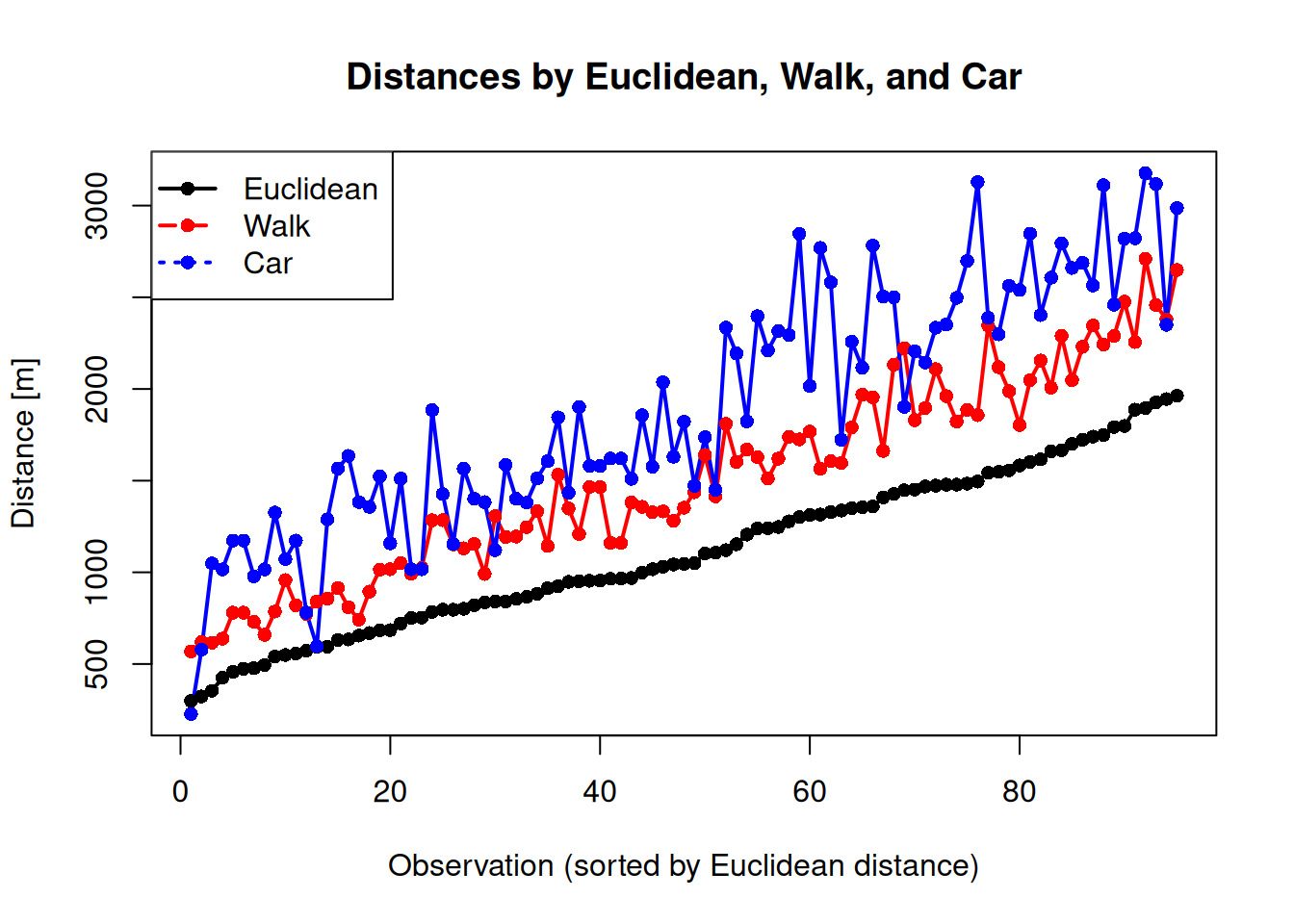
)We can now compare the euclidean and routing distances that we estimated for the survey locations under 2 km.
summary(SURVEYsample$distance) # Euclidean Min. 1st Qu. Median Mean 3rd Qu. Max.
298 790 1046 1112 1470 1963 summary(SURVEYwalk$distance) # Walk Min. 1st Qu. Median Mean 3rd Qu. Max.
569 1090 1465 1505 1925 2710 summary(SURVEYcar$distance) # Car Min. 1st Qu. Median Mean 3rd Qu. Max.
228 1401 1823 1893 2431 3177 What can you understand from this results?
Compare 1 single route.
mapview(SURVEYeuclidean[165,], color = "black") + # 1556 meters
  mapview(SURVEYwalk[78,], color = "red") + # 1989 meters
  mapview(SURVEYcar[78,], color = "blue") # 2565 meters
With this we can see the circuity of the routes, a measure of route / transportation efficiency, which is the ratio between the routing distance and the euclidean distance.
The cicuity for car (1.65) is usually higher than for walking (1.28) or biking, for shorter distances.
Visualize with transparency of 30%, to get a clue when they overlay.
mapview(SURVEYwalk, alpha = 0.3)mapview(SURVEYcar, alpha = 0.3, color = "red")We can also use the overline() function from stplanr package to break up the routes when they overline, and add them up.
# we create a value that we can later sum
# it can be the number of trips represented by this route
SURVEYwalk$trips = 1 # in this case is only one respondent per route

SURVEYwalk_overline = stplanr::overline(
  SURVEYwalk,
  attrib = "trips",
  fun = sum
)

mapview(SURVEYwalk_overline, zcol = "trips", lwd = 3)
With this we can visually inform on how many people travel along a route, from the survey dataset2.