Code
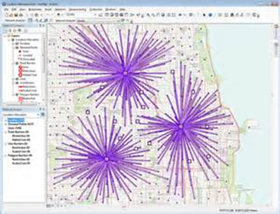
TRIPSmode = readRDS("data/TRIPSmode.Rds")Desire lines are a way to represent the flow of people or goods between two points. They are often used in transport planning to represent the flow of trips between zones.
There are many ways to create desire lines, connecting origins and destinations. For instance:
1 origin to 1 destination
multiple origins to a single destinations
origin zone to destination zone
OD jittering1
The stplanr package is a collection of functions for sustainable transport planning with R, and it is built on top of the sf package (Lovelace and Ellison 2018).
In this workshop, we will use the od package, a lightweight package with a few functions from stplanr, namely the ones to create desire lines from origin-destination (OD) pairs (Lovelace and Morgan 2024).
od_to_sfTo create desire lines, we need a dataset with OD pairs and other dataset with the corresponding transport zones (spatial data).
The TRIPSmode.Rds dataset includes origins, destinations and number of trips between municipalities.
TRIPSmode = readRDS("data/TRIPSmode.Rds")The Municipalities_geo.gpkg dataset includes the geometry of the transport zones.
library(sf)
Municipalities_geo = st_read("data/Municipalities_geo.gpkg", quiet = TRUE) # supress mesage
Then, we need to load the od package. We will use the od_to_sf() function to create desire lines from OD pairs.
# install.packages("od")
library(od)

TRIPSdlines = od_to_sf(TRIPSmode, z = Municipalities_geo) # z for zones
For this magic to work smoothly, the first two columns of the TRIPSmode dataset must be the origin and destination zones, and these zones need to correspond to the first column of the Municipalities_geo dataset (with an associated geometry).
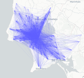
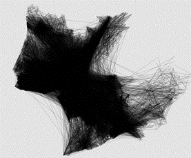
Now we can visualize the desire lines using the mapview function.
library(mapview)
mapview(TRIPSdlines, zcol = "Total")
As you can see, this is too much information to be able to understand the flows.
Filter intrazonal trips.
library(dplyr)

TRIPSdlines_inter = TRIPSdlines |>
  filter(Origin != Destination) |> # remove intrazonal trips
  filter(Total > 5000) # remove noise

mapview(TRIPSdlines_inter, zcol = "Total", lwd = 5)
Filter trips with origin or destination not in Lisbon.
TRIPSdl_noLX = TRIPSdlines_inter |>
  filter(Origin != "Lisboa", Destination != "Lisboa")

mapview(TRIPSdl_noLX, zcol = "Total", lwd = 8) # larger line width
Try to replace the Total with other variables, such as Car, PTransit, and see the differences.
Note that the od_to_sf() function creates bidirectional desire lines. This can be not the ideal for visualization / representation purposes, as you will have 2 lines overlaping.
The function od_oneway() aggregates oneway lines to produce bidirectional flows.
By default, it returns the sum of each numeric column for each bidirectional origin-destination pair.
nrow(TRIPSdlines)[1] 315TRIPSdlines_oneway = od_oneway(TRIPSdlines) |>
filter(o != d) # remove empty geometries
nrow(TRIPSdlines_oneway)[1] 150Note that for the last municipalities you have less combinations now. Nevertheless, all the possible combinations are represented.
head(TRIPSdlines_oneway[,c(1,2)]) # just the first 2 columnsSimple feature collection with 6 features and 2 fields
Attribute-geometry relationships: identity (2)
Geometry type: LINESTRING
Dimension: XY
Bounding box: xmin: -9.229502 ymin: 38.62842 xmax: -8.91588 ymax: 38.75981
Geodetic CRS: WGS 84
o d geometry
1 Alcochete Almada LINESTRING (-8.91588 38.735...
2 Alcochete Amadora LINESTRING (-8.91588 38.735...
3 Almada Amadora LINESTRING (-9.193069 38.63...
4 Alcochete Barreiro LINESTRING (-8.91588 38.735...
5 Almada Barreiro LINESTRING (-9.193069 38.63...
6 Amadora Barreiro LINESTRING (-9.229502 38.75...tail(TRIPSdlines_oneway[,c(1,2)])Simple feature collection with 6 features and 2 fields
Attribute-geometry relationships: identity (2)
Geometry type: LINESTRING
Dimension: XY
Bounding box: xmin: -9.357651 ymin: 38.4949 xmax: -8.806644 ymax: 38.92211
Geodetic CRS: WGS 84
o d geometry
145 Oeiras Vila Franca de Xira LINESTRING (-9.276317 38.71...
146 Palmela Vila Franca de Xira LINESTRING (-8.806644 38.61...
147 Seixal Vila Franca de Xira LINESTRING (-9.108801 38.60...
148 Sesimbra Vila Franca de Xira LINESTRING (-9.120124 38.49...
149 Setúbal Vila Franca de Xira LINESTRING (-8.887481 38.51...
150 Sintra Vila Franca de Xira LINESTRING (-9.357651 38.82...Example of visualization with Public Transit trips in both ways.
TRIPSdlines_oneway_noLX = TRIPSdlines_oneway |>
  filter(PTransit > 5000) # reduce noise

mapview(TRIPSdlines_oneway_noLX, zcol = "PTransit", lwd = 8)The od_to_sf() function uses the geometric center of the zones to create the desire lines. But if we replace those zones by the weighted centroids, we can have a more realistic representation of the flows.
# Centroid_pop = st_read("data/Centroid_pop.gpkg")

TRIPSdlines_pop = od_to_sf(TRIPSmode, z = Centroid_pop) |>  # works the same way
  od_oneway() |> # oneway
  filter(o != d) # remove empty geometries
Check differences of lines with trips from/to Lisbon:
TRIPSdlines_geo_LX = TRIPSdlines_oneway |>
  filter(o == "Lisboa" | d == "Lisboa") # or condition
TRIPSdlines_pop_LX = TRIPSdlines_pop |>
  filter(o == "Lisboa" | d == "Lisboa")

mapview(TRIPSdlines_geo_LX, color = "blue") + mapview(TRIPSdlines_pop_LX, color = "red")
The next step will be estimating the euclidean distances between these centroids, and compare them with the routing distances.