Code
library(dplyr)
library(sf)
library(mapview)
Municipalities_geo = st_read("data/Municipalities_geo.gpkg", quiet = TRUE)
Centroids_geo = st_centroid(Municipalities_geo)In this section we will calculate the geometric and the weighted centroids of transport zones.
Taking the Municipalities_geo data from the previous section, we will calculate the geometric centroids, using the st_centroid() function.
library(dplyr)
library(sf)
library(mapview)
Municipalities_geo = st_read("data/Municipalities_geo.gpkg", quiet = TRUE)
Centroids_geo = st_centroid(Municipalities_geo)This creates points at the geometric center of each polygon.
mapview(Centroids_geo)mapview(Centroids_geo) + mapview(Municipalities_geo, alpha.regions = 0) # both maps, with full transparency in polygonsBut… is this the best way to represent the center of a transport zone?
These results may be biased by the shape of the polygons, and not represent where activities are. Example: lakes, forests, etc.
To overcome this, we can use weighted centroids.
We will weight centroids of transport zones by population and by number of buildings.
For this, we will need the census data (INE 2022).
Census = st_read("data/census.gpkg", quiet = TRUE)
mapview(Census |> filter(Municipality == "Lisboa"), zcol = "Population")It was not that easy to estimate weighted centroids with R, as it is with GIS software. But there is this new package centr that can help us (Zomorrodi 2024).
We need to specify the group we want to calculate the mean centroids, and the weight variable we want to use.
# test
library(centr)
Centroid_pop = Census |>
mean_center(group = "Municipality", weight = "Population")We can do the same for buildings.
Centroid_build = Census |>
mean_center(group = "Municipality", weight = "Buildings")mapview(Centroids_geo, col.region = "blue") +
mapview(Centroid_pop, col.region = "red") +
mapview(Centroid_build, col.region = "black") +
mapview(Municipalities_geo, alpha.regions = 0) # polygon limitsSee how the building, population and geometric centroids of Sintra are apart, from closer to Tagus, to the rural area.
To produce the same map, using only plot() and st_geometry(), we need to make sure that the geometries have the same crs.
st_crs(Centroids_geo) # 4326 WGS84
st_crs(Centroid_pop) # 3763 Portugal TM06So, we need to transform the geometries to the same crs.
Centroid_pop = st_transform(Centroid_pop, crs = 4326)
Centroid_build = st_transform(Centroid_build, crs = 4326)Now, to use plot() we incrementally add layers to the plot.
# Plot the Municipalities_geo polygons first (with no fill)
plot(st_geometry(Municipalities_geo), col = NA, border = "black")
# Add the Centroids_geo points in blue
plot(st_geometry(Centroids_geo), col = "blue", pch = 16, add = TRUE) # add!
# Add the Centroid_pop points in red
plot(st_geometry(Centroid_pop), col = "red", pch = 16, add = TRUE)
# Add the Centroid_build points in black
plot(st_geometry(Centroid_build), col = "black", pch = 16, add = TRUE)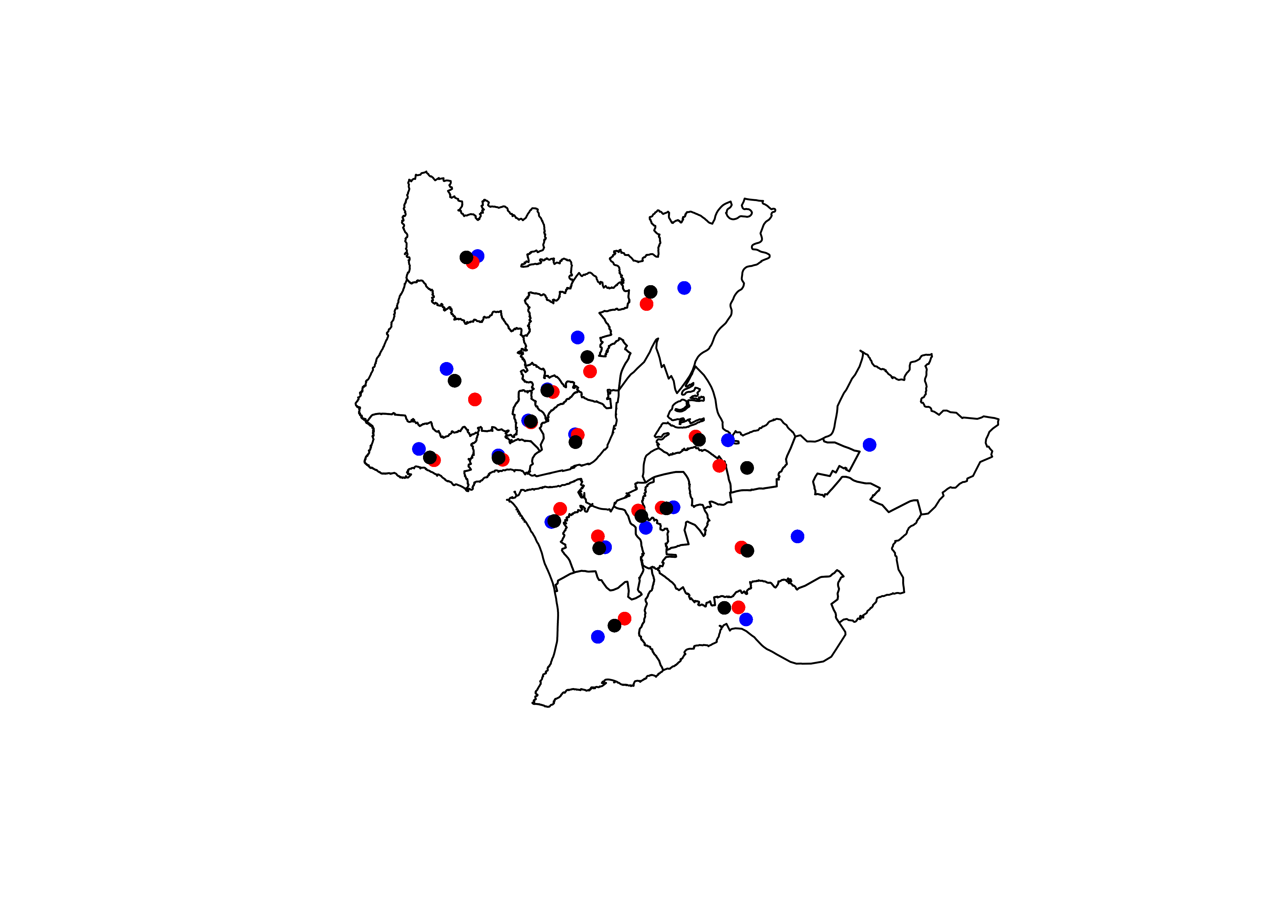
In the next section we will use these centroids to calculate the desire lines between them.