# library(tidyverse)
library(dplyr)5 Data manipulation
In this chapter we will use some very useful dplyr functions to handle and manipulate data.
You can load the dplyr package directly, or load the entire tidy universe (tidyverse).
Using the same dataset as in R basics but with slightly differences1.
We will do the same operations but in a simplified way.
TRIPS = readRDS("data/TRIPSorigin.Rds")
Important
Note that it is very important to understand the R basics, that’s why we started from there, even if the following functions will provide the same results.
You don’t need to know everything! And you don’t need to know by heart. The following functions are the ones you will probably use most of the time to handle data.
There are several ways to reach the same solution. Here we present only one of them.
5.1 Select variables
Have a look at your dataset. You can open using View(), look at the information at the “Environment” panel, or even print the same information using glimpse()
glimpse(TRIPS)We will create a new dataset with Origin, Walk, Bike and Total. This time we will use the select() function.
TRIPS_new = select(TRIPS, Origin, Walk, Bike, Total) # the first argument is the datasetThe first argument, as usually in R, is the dataset, and the remaining ones are the columns to select.
With most of the dplyr functions you don’t need to refer to data$... you can simply type the variable names (and even without the "..."!). This makes coding in R simpler :)
You can also remove columns that you don’t need.
TRIPS_new = select(TRIPS_new, -Total) # dropping the Total column5.1.1 Using pipes!
Now, let’s introduce pipes. Pipes are a rule as: “With this, do this.”
This is useful to skip the first argument of the functions (usually the dataset to apply the function).
Applying a pipe to the select() function, we can write as:
TRIPS_new = TRIPS |> select(Origin, Walk, Bike, Total)Two things to note:
The pipe symbol can be written as
|>or%>%. 2 To write it you may also use thectrl+shift+mshortcut.After typing
select(you can presstaband the list of available variables of that dataset will show up!Enterto select. With this you prevent typo errors.
5.2 Filter observations
You can filter observations based on a condition using the filter() function.
TRIPS2 = TRIPS[TRIPS$Total > 25000,] # using r-base, you cant forget the comma
TRIPS2 = TRIPS2 |> filter(Total > 25000) # using dplyr, it's easier
You can have other conditions inside the condition.
summary(TRIPS$Total) Min. 1st Qu. Median Mean 3rd Qu. Max.
361 5918 17474 22457 33378 112186 TRIPS3 = TRIPS |> filter(Total > median(Total)) Other filter conditions:
==equal,!=different<smaller,>greater,<=smaller or equal,>=greater or equal&and,|oris.na,!is.nais not NA%in%,!%in%not in
5.3 Create new variables
You can also try again to create a variable of Car percentage using pipes! To create a new variable or change an existing one (overwriting), you can use the mutate() function.
TRIPS$Car_perc = TRIPS$Car/TRIPS$Total * 100 # using r-base

TRIPS = TRIPS |> mutate(Car_perc = Car/Total * 100) # using dplyr
5.4 Change data type
Data can be in different formats. For example, the variable Origin is a character, but we can convert it to a numeric variable.
class(TRIPS$Origin)[1] "character"TRIPS = TRIPS |>
mutate(Origin_num = as.integer(Origin)) # you can use as.numeric() as well
class(TRIPS$Origin_num)[1] "integer"Most used data types are:
- integer (
int) - numeric (
num) - character (
chr) - logical (
logical) - date (
Date) - factor (
factor)
5.4.1 Factors
Factors are useful to deal with categorical data. You can convert a character to a factor using as.factor(), and also use labels and levels for categorical ordinal data.
We can change the Lisbon variable to a factor, and Internal too.
TRIPS = TRIPS |>
  mutate(Lisbon_factor = factor(Lisbon, labels = c("No", "Yes")),
         Internal_factor = factor(Internal, labels = c("Inter", "Intra")))
But how do we know which levels come first? A simple way is to use table() or unique() functions.
unique(TRIPS$Lisbon) # this will show all the different values[1] 0 1table(TRIPS$Lisbon) # this will show the frequency of each value
  0   1
188 48 table(TRIPS$Lisbon_factor)
 No Yes
188  48
The first number to appear is the first level, and so on.
You can see the difference between using a continuous variable (in this case Lisbon` has 0 and 1) and a categorical variable (Lisbon_factor).
plot(TRIPS$Lisbon) # the values range between 0 and 1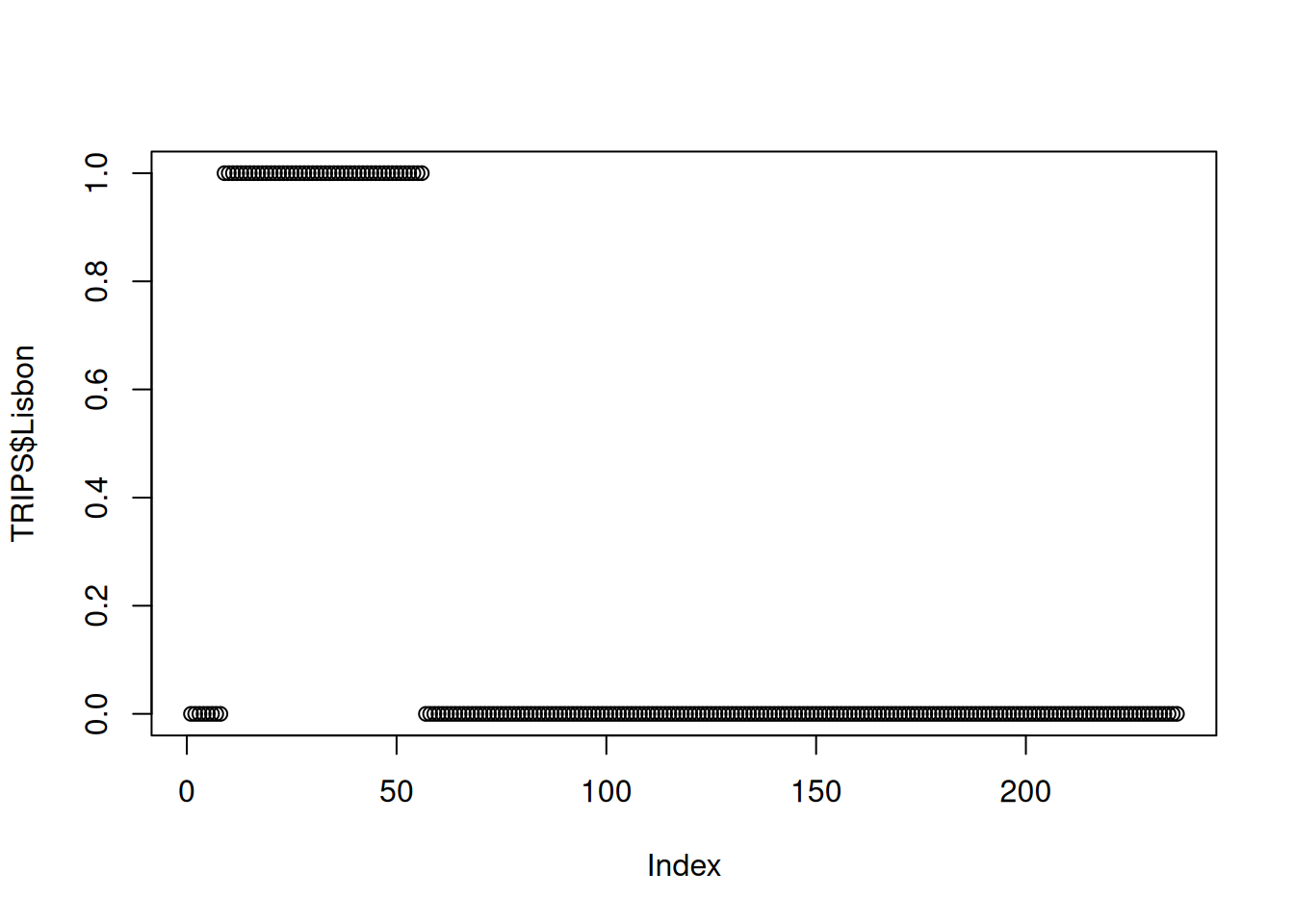
plot(TRIPS$Lisbon_factor) # the values are categorical and labeled with Yes/No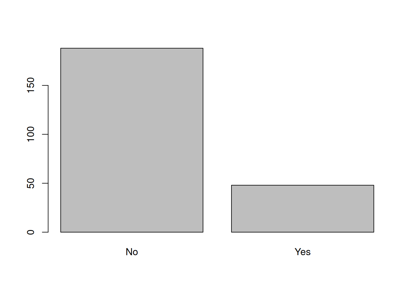
5.5 Join data tables
When having relational tables - i.e. with a common identifier - it is useful to be able to join them in a very efficient way.
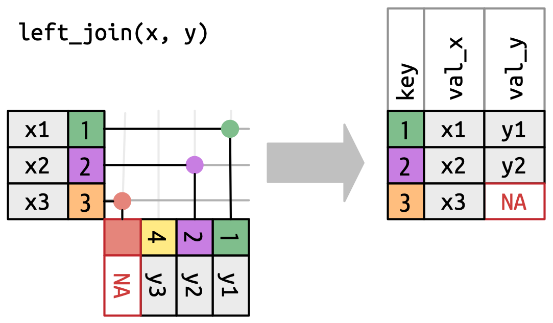
left_join is a function that joins two tables by a common column. The first table is the one that will be kept, and the second one will be joined to it. How left_join works:
Let’s join the municipalities to this table with a supporting table that includes all the relation between neighbourhoods and municipalities, and the respective names and codes.
Municipalities = readRDS("data/Municipalities_names.Rds")head(TRIPS)# A tibble: 6 × 13
Origin Total Walk Bike Car PTransit Other Internal Lisbon Car_perc
<chr> <dbl> <dbl> <dbl> <dbl> <dbl> <dbl> <dbl> <dbl> <dbl>
1 110501 35539 11325 1309 21446 1460 0 0 0 60.3
2 110501 47602 3502 416 37727 5519 437 1 0 79.3
3 110506 37183 12645 40 22379 2057 63 0 0 60.2
4 110506 42313 1418 163 37337 3285 106 1 0 88.2
5 110507 30725 9389 1481 19654 201 0 0 0 64.0
6 110507 54586 2630 168 44611 6963 215 1 0 81.7
# ℹ 3 more variables: Origin_num <int>, Lisbon_factor <fct>,
# Internal_factor <fct>tail(Municipalities) Mun_code Neighborhood_code Municipality
113 1109 110913 Mafra
114 1114 111409 Vila Franca de Xira
115 1109 110918 Mafra
116 1109 110904 Mafra
117 1502 150202 Alcochete
118 1109 110911 Mafra
Neighborhood
113 Santo Isidoro
114 Vila Franca de Xira
115 União das freguesias de Azueira e Sobral da Abelheira
116 Encarnação
117 Samouco
118 MilharadoWe can see that we have a common variable: Origin in TRIPS and Neighborhood_code in Municipalities.
To join these two tables we need to specify the common variable in each table, using the by argument.
TRIPSjoin = TRIPS |> left_join(Municipalities, by = c("Origin" = "Neighborhood_code"))If you prefer, you can mutate or rename a variable so both tables have the same name. When both tables have the same name, you don’t need to specify the by argument.
Municipalities = Municipalities |> rename(Origin = "Neighborhood_code") # change name
TRIPSjoin = TRIPS |> left_join(Municipalities) # automatic detects common variable
As you can see, both tables don’t need to be the same length. The left_join function will keep all the observations from the first table, and join the second table to it. If there is no match, the variables from the second table will be filled with NA.
5.6 group_by and summarize
We have a very large table with all the neighbourhoods and their respective municipalities. We want to know the total number of trips with origin in each municipality.
To make it easier to understand, let’s keep only the variables we need.
TRIPSredux = TRIPSjoin |> select(Origin, Municipality, Internal, Car, Total)
head(TRIPSredux)
# A tibble: 6 × 5
Origin Municipality Internal Car Total
<chr> <chr> <dbl> <dbl> <dbl>
1 110501 Cascais 0 21446 35539
2 110501 Cascais 1 37727 47602
3 110506 Cascais 0 22379 37183
4 110506 Cascais 1 37337 42313
5 110507 Cascais 0 19654 30725
6 110507 Cascais 1 44611 54586We can group this table by the Municipality variable and summarize the number of trips with origin in each municipality.
TRIPSsum = TRIPSredux |>
  group_by(Municipality) |> # you won't notice any chagne with only this
  summarize(Total = sum(Total))
head(TRIPSsum)
# A tibble: 6 × 2
Municipality Total
<chr> <dbl>
1 Alcochete 36789
2 Almada 289834
3 Amadora 344552
4 Barreiro 133658
5 Cascais 373579
6 Lisboa 1365111We summed the total number of trips in each municipality.
If we want to group by more than one variable, we can add more group_by() functions.
TRIPSsum2 = TRIPSredux |>
  group_by(Municipality, Internal) |>
  summarize(Total = sum(Total),
            Car = sum(Car))
head(TRIPSsum2)
# A tibble: 6 × 4
# Groups: Municipality [3]
Municipality Internal Total Car
<chr> <dbl> <dbl> <dbl>
1 Alcochete 0 16954 9839
2 Alcochete 1 19835 15632
3 Almada 0 105841 49012
4 Almada 1 183993 125091
5 Amadora 0 117727 33818
6 Amadora 1 226825 142386We summed the total number of trips and car trips in each municipality, separated by inter and intra municipal trips.
It is a good practice to use the ungroup() function after the group_by() function. This will remove the grouping. If you don’t do this, the grouping will be kept and you may have unexpected results in the next time you use that dataset.
5.7 Arrange data
You can sort a dataset by one or more variables.
For instance, arrange() by Total trips, ascending or descending order.
TRIPS2 = TRIPSsum2 |> arrange(Total)
TRIPS2 = TRIPSsum2 |> arrange(-Total) # descending

TRIPS2 = TRIPSsum2 |> arrange(Municipality) # alphabetic

TRIPS4 = TRIPS |> arrange(Lisbon_factor, Total) # more than one variable
This is not the same as opening the view table and click on the arrows. When you do that, the order is not saved in the dataset. If you want to save the order, you need to use the arrange() function.
5.8 All together now!
This is the pipes magic. It takes the last result and applies the next function to it. “With this, do this.”. You can chain as many functions as you want.
TRIPS_pipes = TRIPS |>
  select(Origin, Internal, Car, Total) |>

  mutate(Origin_num = as.integer(Origin)) |>
  mutate(Internal_factor = factor(Internal, labels = c("Inter", "Intra"))) |>

  filter(Internal_factor == "Inter")|>

  left_join(Municipalities) |>

  group_by(Municipality) |>
  summarize(Total = sum(Total),
            Car = sum(Car),
            Car_perc = Car/Total * 100) |>
  ungroup() |>

  arrange(desc(Car_perc))
With this code we will have a table with the total number of intercity trips, by municipality, with their names instead of codes, arranged by the percentage of car trips.
TRIPS_pipes# A tibble: 18 × 4
Municipality Total Car Car_perc
<chr> <dbl> <dbl> <dbl>
1 Mafra 65811 46329 70.4
2 Sesimbra 49370 31975 64.8
3 Cascais 161194 96523 59.9
4 Palmela 66428 39688 59.7
5 Alcochete 16954 9839 58.0
6 Setúbal 129059 70318 54.5
7 Montijo 57164 30900 54.1
8 Seixal 120747 63070 52.2
9 Sintra 237445 123408 52.0
10 Oeiras 134862 66972 49.7
11 Almada 105841 49012 46.3
12 Loures 132310 60478 45.7
13 Barreiro 52962 24160 45.6
14 Odivelas 93709 39151 41.8
15 Vila Franca de Xira 115152 47201 41.0
16 Moita 51040 17394 34.1
17 Amadora 117727 33818 28.7
18 Lisboa 280079 69038 24.65.9 Other dplyr functions
You can explore other dplyr functions and variations to manipulate data in the dplyr cheat sheet:
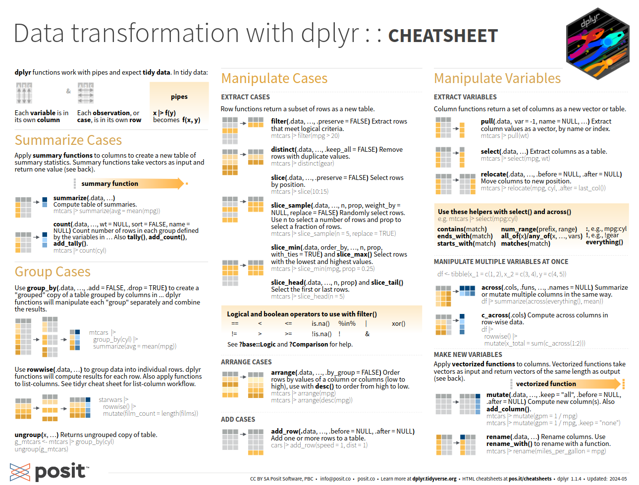
Take a particular attention to pivot_wider and pivot_longer (tidyr package) to transform OD matrices in wide and long formats.
| Origins | Destinations | Trips |
|---|---|---|
| A | B | 20 |
| A | C | 45 |
| B | A | 10 |
| C | C | 5 |
| C | A | 30 |
| Trips | A | B | C |
|---|---|---|---|
| A | NA | 20 | 45 |
| B | 10 | NA | NA |
| C | 30 | NA | 5 |