POIs and Grids

Census data

Search and download your census data from official sources.

In Portugal: https://mapas.ine.pt/download/index2021.phtml

For this exercises, you just need the population associated with a statistical unit, as smaller as possible

library(tidyverse)
library(sf)

census = st_read("data/Lisbon/BGRI2021_1106.gpkg") # census units in polygons
plot(census$geom)

# from polygons to points
census_poitns = census |> 
  st_transform(4326) |> # make sue it is in universal CRS
  st_centroid()
plot(census_poitns) # census units in points
names(census_poitns)

census_poitns = census_poitns |>
  select(BGRI2021, N_INDIVIDUOS) |> # only my code area and population
  rename(id = BGRI2021,
         residents = N_INDIVIDUOS) # rename variables
st_write(census_poitns, "data/census_poitns.gpkg") # save for later

Code

library(mapview)
mapview(census_poitns) + mapview(census)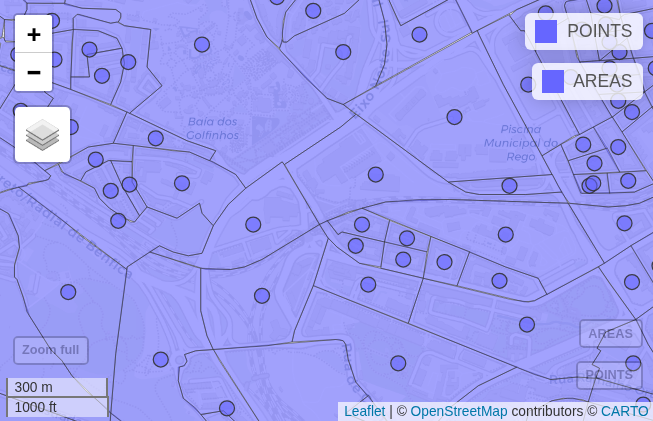

Dissolve - City limit

In the case you don’t have already a city limit, you can create one based on the “dissolve” of the inner boundaries of your census data, as follows

#dissolve 
city_limit = census |> st_union() |> st_as_sf()
plot(city_limit)

Note

If you don’t have census data at a reasonable level (census blocks), you can recreate random points in your city. See the code bellow 🔎

Generate synthetic census-like points for a City

# 0. Load libraries
library(sf)
library(dplyr)

# 1. Read city polygon (replace with your file path)
city_limit <- st_read("data/city_limit.gpkg") |> st_transform(4326)

# 2. Set parameters
set.seed(42) # for reproducibility
total_pop <- 545000 # your city population
avg_residents <- 300 # a census block average
n_points <- round(total_pop / avg_residents)

# 3. Generate random points within the city boundary
census_syn <- st_sample(city_limit, size = n_points, type = "random") |>
  st_as_sf() |>
  mutate(id = 1:n_points)

# # 4. Compute distance from city center (for density weighting) - OPTIONAL
# center <- st_centroid(city_limit)
# dist_center <- as.numeric(st_distance(census_syn, center))  # in meters
# 
# # 5. Create weights so closer points get higher population - OPTIONAL
# # Inverse distance weighting (add +1 to avoid division by zero)
# weights <- 1 / (dist_center + 1)

# assign random populations that sum to total_pop
weights <- runif(n_points)

# Normalize weights to sum to 1 and assign residents
residents <- round(weights / sum(weights) * total_pop)

# 6. Adjust rounding so the total sums exactly to total_pop
diff <- total_pop - sum(residents)
if (diff != 0) {
  residents[1:abs(diff)] <- residents[1:abs(diff)] + sign(diff)
}

# 7. Add residents to points
census_syn$residents <- residents
sum(census_syn$residents) # should be total_pop

# 8. Quick visualization
mapview::mapview(census_syn, zcol = "residents")

# 9. Save for later
st_write(census_syn, "data/synthetic_census_points.gpkg", delete_dsn = TRUE)

Points of Interest

OpenStreetMap

From OSM we can export several different opportunities to use on routing and accessibility exercises.

For instance, the 15-min city idea follows the Flowers of Proximity, to categorize the opportinities in 7 different categories, based on Büttner et al. (2022).

For the Streets4All project, and SiteSelection package (Rosa Félix and Gabriel Valença 2024), we divided in:

Amenities
Healthcare
Leisure
Shop
Sport
Tourism

Hot export tool

Using the HOT Export Tool, you can select a few categories, and export as .gpkg or .geojson.

Select 6 to 8 categories

For instance: schools, hospitals, ATMs, parks, supermarkets, and restaurants.

Your further analysis will be made by comparing the categories you selected and exported.

Dealing with points and polygons from OSM

If your export brings both polygons and points, you should convert the polygons to points (centroids).

pois_raw = st_read("data/pois.gpkg") # downloaded from HOT export

pois_cat = pois_raw |> 
  mutate(type = case_when(
      !is.na(shop) & shop %in% c("supermarket", "convenience") ~ "grocery",
      amenity == "marketplace" ~ "grocery",
      !is.na(leisure) ~ leisure,
      amenity %in% c("restaurant", "pub", "cafe", "bar", "fast_food") ~ "restaurant",
      TRUE ~ amenity
    )) |> 
  select(osm_id, type, name)

table(pois_cat$type)

       atm    grocery   hospital       park restaurant     school 
       316        799         42        503       4956        445

# separate points form polygons
pois_points = pois_cat |> st_collection_extract("POINT")
pois_polygons = pois_cat |>  st_collection_extract("POLYGON")

# transform polygons in points
pois_polygons = st_centroid(pois_polygons)

# bind them
pois = bind_rows(pois_points, pois_polygons)

mapview(pois, zcol = "type")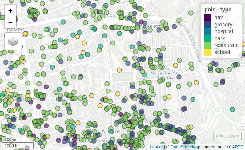

Geometric filter

To keep only the POIs relative to your city limit, you can make a geometrical filter, as:

pois = pois[city_limit,]

# export for later
st_write(pois, "data/Lisbon/pois_osm_points.gpkg", delete_dsn = TRUE)

Script

A more flexible approach to download the data, but requires more codding 🧑‍💻

See the script we did for all Portugal, and the dataset for Lisbon (2024): data_extract.R (line 146)

You can explore other OpenStreetMap categories at their Wiki.

Grids

You may want to use the original census units, or create a squared oh hexagonal grid.

Create a grid
Match all the Census and POIs to that grid

Create a grid

We will use the city of Lisbon as example

library(sf)
library(tidyverse)
library(mapview)

city_limit = st_read("data/Lisbon/Lisboa_lim.gpkg")
plot(city_limit)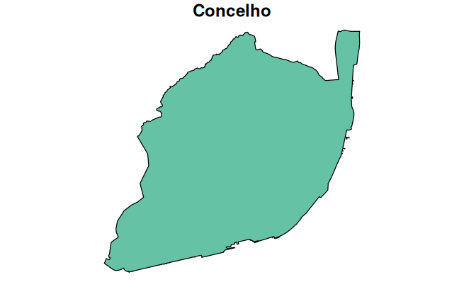

Hexagonal using `h3jsr`

Make an hexagonal grid that covers the city polygon, using the universal H3 grid.

library(h3jsr)

# Resolution: https://h3geo.org/docs/core-library/restable/ 
# h3_res = 10 # 150m diameter
h3_res = 9 # 400m diameter
# h3_res = 8 # 1060m diameter

GRID_h3 = city_limit |>  
  polygon_to_cells(res = h3_res, simple = FALSE)
GRID_h3 = GRID_h3$h3_addresses |>
  cell_to_polygon(simple = FALSE)
GRID_h3 = GRID_h3 |>
  mutate(id = seq(1:nrow(GRID_h3)))  # give an ID to each cell
h3_index = GRID_h3 |> st_drop_geometry() # save h3_address for later

mapview(GRID_h3)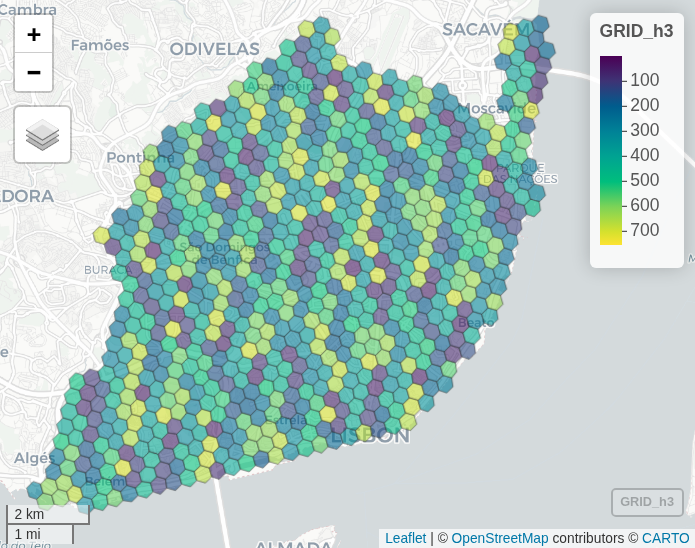

Squared

Make a squared grid that covers the city polygon

GRID = city_limit |>
  st_transform(crs = 3857) |> # to a projected crs
  st_make_grid(cellsize = 400, # meters, we are using a projected crs
               what = "polygons",
               square = TRUE) |> # if FALSE, hexagons
  st_sf() |> # from list to sf
  st_transform(crs = 4326) |>  # back to WGS84
  st_intersection(city_limit$geom) # crop (optional)

GRID = GRID |>  
  rename(geometry = st_make_grid.st_transform.city_limit..crs...3857...cellsize...400..) |> 
  mutate(id = c(1:nrow(GRID))) # just to give an ID to each cell 
  
mapview(GRID, alpha.regions = 0.2)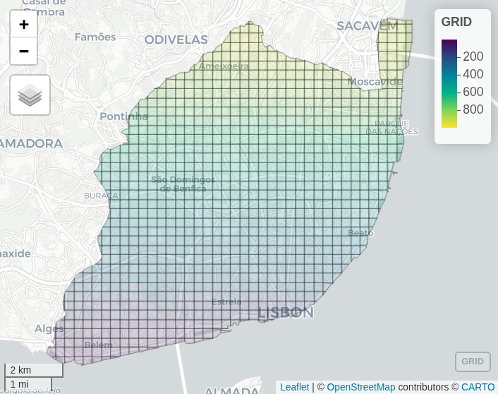

Tip

You should stick with just one of them: squares or hexagons.

Areas with information

Now, we can associate these areas (and their centroids) with all the information we want.

With POIs

# Points of interest from script
POIs = st_read("https://github.com/U-Shift/Traffic-Simulation-Models/releases/download/2025/pois_osm_points.gpkg")

Code for squares

# count points by type in areas
GRID_pois = POIs |> st_join(GRID, join = st_within)

counts_type = GRID_pois |>
     st_drop_geometry() |>   # drop geometry for counting
     group_by(id, type) |>
     summarise(n = n(), .groups = "drop") |>
     tidyr::pivot_wider(names_from = type, values_from = n, values_fill = 0)

GRID_pois = GRID |>
  left_join(counts_type, by = "id") |>
  mutate(across(where(is.numeric), ~replace_na(.x, 0)))

mapview(GRID_pois, zcol = "restaurant") # for instance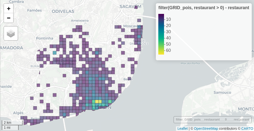

The result is a grid with too many columns (one for each type). Consider using only the group.

With Census

# Census data
census = st_read("https://github.com/U-Shift/Traffic-Simulation-Models/releases/download/2025/Censos_Lx.gpkg")

# count points by type in areas
GRID_census = census |> st_join(GRID, join = st_within)

census_density = GRID_census |>
  st_drop_geometry() |>   # drop geometry for counting
  group_by(id.y) |>
  summarise(buildings = sum(buildings),
            families = sum(families),
            residents = sum(residents)) |> 
  rename(id = id.y) |> 
  filter(!is.na(id))

GRID_census = GRID |>
  left_join(census_density, by = "id") |>
  mutate(across(where(is.numeric), ~replace_na(.x, 0)))

mapview(GRID_census, zcol = "residents")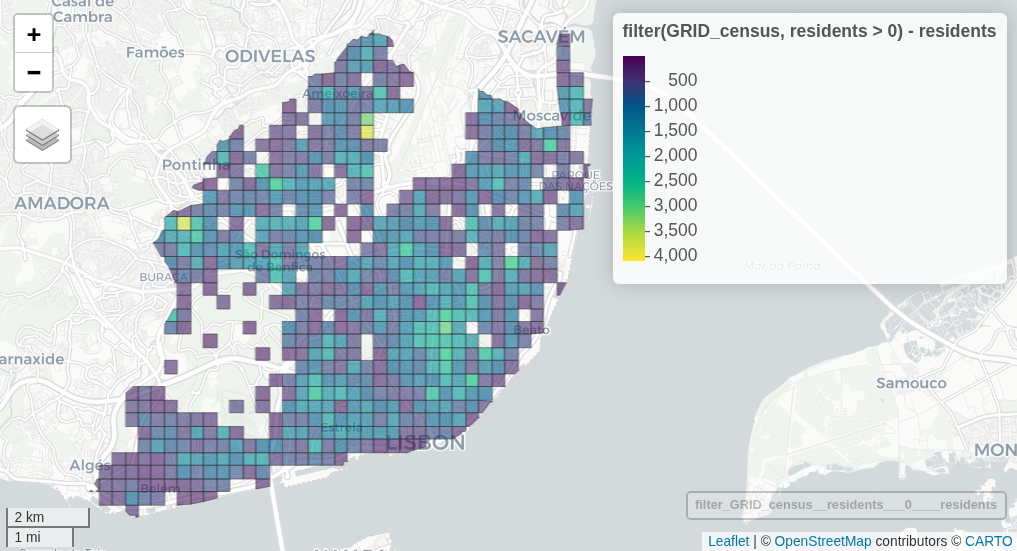

All together

GRID_data = GRID_census |> left_join(GRID_pois |> st_drop_geometry())

The same for Hex grid

Code for Hexagons

# POIs
GRIDhex_pois = POIs |> st_join(GRID_h3, join = st_within)

counts_type = GRIDhex_pois |>
     st_drop_geometry() |>   # drop geometry for counting
     group_by(id, type) |>
     summarise(n = n(), .groups = "drop") |>
     tidyr::pivot_wider(names_from = type, values_from = n, values_fill = 0)

GRIDhex_pois = GRID_h3 |>
  left_join(counts_type, by = "id") |>
  mutate(across(where(is.numeric), ~replace_na(.x, 0)))

#  Census
GRIDhex_census = census |> st_join(GRID_h3, join = st_within)

census_density = GRIDhex_census |>
  st_drop_geometry() |>   # drop geometry for counting
  group_by(id.y) |>
  summarise(buildings = sum(buildings),
            families = sum(families),
            residents = sum(residents)) |> 
  rename(id = id.y) |> 
  filter(!is.na(id))

GRIDhex_census = GRID_h3 |>
  left_join(census_density, by = "id") |>
  mutate(across(where(is.numeric), ~replace_na(.x, 0)))

# All together now
GRIDhex_data = GRIDhex_census |> left_join(GRIDhex_pois |> st_drop_geometry())

mapview(GRIDhex_data, zcol = "residents")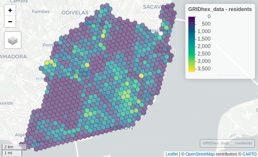

Centroid coordinates

We may want to have this information as points, for instance for routing to opportunities.

# hexagons
POINTShex = GRIDhex_data |> 
  st_centroid()
GRIDhex_data = GRIDhex_data |> 
  mutate(lon = st_coordinates(POINTShex)[,1],
         lat = st_coordinates(POINTShex)[,2])

# squares
POINTSsq = GRID_data |> 
  st_centroid()
GRID_data = GRID_data |> 
  mutate(lon = st_coordinates(POINTSsq)[,1],
         lat = st_coordinates(POINTSsq)[,2])

Tip

Don’t forget to save your data, this will be very useful for the next exercises.

saveRDS(GRID_data, "data/Lisbon/GRIDsq_data.rds")
saveRDS(GRIDhex_data, "data/Lisbon/GRIDhex_data.rds")

References

Büttner, Benjamin, Sebastian Seisenberger, María Teresa Baquero Larriva, Ana Graciela Rivas De Gante, Sindi Haxhija, Alba Ramirez, and Bartosz McCormick. 2022. “±15-Minute City: Human-centred planning in action - Mobility for more liveable urban spaces.” Munich: EIT Urban Mobility, Technical University of Munich. https://www.eiturbanmobility.eu/wp-content/uploads/2022/11/EIT-UrbanMobilityNext9_15-min-City_144dpi.pdf.

Rosa Félix, and Gabriel Valença. 2024. SiteSelection: An r Script to Find Complex Areas for the Streets4All Project. https://u-shift.github.io/SiteSelection/.

Census data

Dissolve - City limit

Points of Interest

OpenStreetMap

Hot export tool

Dealing with points and polygons from OSM

Geometric filter

Script

Grids

Create a grid

Hexagonal using h3jsr

Squared

Areas with information

With POIs

With Census

All together

Centroid coordinates

References

Hexagonal using `h3jsr`