Pareto frontier

Fares and accessibility

See the r5r vignettes “Accounting for monetary costs” and “Trade-offs between travel time and monetary cost” (Pereira et al. 2021)

Create rules for an operator

In this case, I am creating random rules for fares, considering the mode, the transfers, and changing between modes.

# create basic fare structure
fare_structure <- setup_fare_structure(r5r_lisboa, 
                                       base_fare = 1.65,
                                       by = "MODE")

# update the cost of bus and subway fares
fare_structure$fares_per_type <- fare_structure$fares_per_type |> 
  mutate(fare = case_when(
    type == "BUS"    ~ 1.65,
    type == "SUBWAY" ~ 2.00, # imagine it is more expensive
    TRUE             ~ fare   # keep existing fare if no condition matches
  ))

# update the cost of transfers
fare_structure$fares_per_transfer <- fare_structure$fares_per_transfer |> 
  mutate(fare = case_when(
    first_leg == "BUS" & second_leg == "BUS" ~ 2.80, # extra cost for 2 trips
      first_leg == "SUBWAY" & second_leg == "SUBWAY" ~ 2.00, # no extra cost
    first_leg != second_leg                  ~ 3.50,
    TRUE                                     ~ fare
  ))


# update transfer_time_allowance to 60 minutes
fare_structure$transfer_time_allowance <- 60

fare_structure$fares_per_type = fare_structure$fares_per_type |>
  mutate(
    unlimited_transfers = if_else(type == "SUBWAY", TRUE, unlimited_transfers),
    allow_same_route_transfer = if_else(type == "SUBWAY", TRUE, allow_same_route_transfer)
  )

# save fare rules to temp file
# r5r::write_fare_structure(fare_structure, file_path = "data/Lisbon/fares_lisbon.zip")
# fare_structure <- r5r::read_fare_structure("data/Lisbon/fares_lisbon.zip")

Calculating a `pareto_frontier()`

In this example, we calculate the Pareto frontier from all origins to downtown (Baixa) considering multiple cutoffs of monetary costs:

€1, which would only allow for walking trips
€1.65, which would only allow for bus trips
€2.00, which would allow for a single or multiple subway trips
€2.80, which would allow for bus + bus
€3.50, which would allow for walking + bus + subway

departure_datetime <- as.POSIXct("01-10-2025 10:00:00", 
                                 format = "%d-%m-%Y %H:%M:%S")

prtf <- pareto_frontier(
  r5r_lisboa,
  origins = POINTS,
  destinations = BAIXA,
  mode = c("WALK", "TRANSIT"),
  departure_datetime = departure_datetime,
  fare_structure = fare_structure,
  fare_cutoffs = c(1, 1.65, 2.0, 2.8, 3.5),
  progress = TRUE
  )

Code

# select some origin and destinations
pf2 <- prtf |> filter(from_id %in% c("727", "1979", "772"))

# recode modes 
pf2 <- pf2 |>
  mutate(
    modes = case_when(
      monetary_cost == 1    ~ "Walk",
      monetary_cost == 1.65 ~ "Bus",
      monetary_cost == 2.0  ~ "Subway",
      monetary_cost == 2.80  ~ "Bus + Bus",
      monetary_cost == 3.5  ~ "Bus + Subway"
      # TRUE                  ~ "Bus"
    )
  )

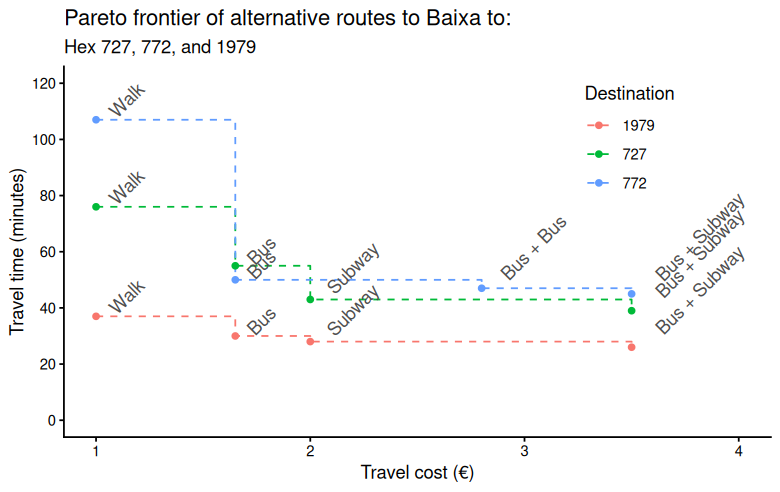
An optimum route alternative means that one cannot make a faster trip without increasing costs, and one cannot make a cheaper trip without increasing travel time.

# calculate travel times function
calculate_travel_times <- function(fare) {
  ttm_df <- travel_time_matrix(
    r5r_lisboa,
    origins = POINTShex,
    destinations = BAIXA,
    mode = c("WALK", "TRANSIT"),
    departure_datetime = departure_datetime,
    time_window = 1,
    fare_structure = fare_structure,
    max_fare = fare,
    max_trip_duration = 60,
    max_walk_time = 15
  )

  return(ttm_df)
}


# calculate travel times, and combine results
ttm <- calculate_travel_times(fare = Inf) # no budget restriction
ttm_200 <- calculate_travel_times(fare = 2) # 2 euro

# merge results
ttm <- ttm |>
  left_join(
    ttm_200 |> select(from_id, to_id, travel_time_p50),
    by = c("from_id", "to_id"),
    suffix = c("", "_200")
  ) |>
  mutate(
    travel_time_200 = travel_time_p50_200,
    travel_time_unl = travel_time_p50
  ) |>
  select(-travel_time_p50, -travel_time_p50_200)


tail(ttm, 10)

Code

# plot of overall travel time differences between limited and unlimited cost travel time matrices 
time_difference <- ttm %>%
  filter(!is.na(travel_time_200)) %>%
  group_by(travel_time_unl, travel_time_200) %>%
  summarise(count = n(), .groups = "drop")

p1 <- ggplot(time_difference, aes(y = travel_time_unl, x = travel_time_200)) +
  geom_point(size = 0.7) +
  coord_fixed() +
  scale_x_continuous(breaks = seq(0, 45, 5)) +
  scale_y_continuous(breaks = seq(0, 45, 5)) +
  theme_light() +
  theme(legend.position = "none") +
  labs(y = "travel time (minutes)\nunestricted monetary cost",
       x = "travel time (minutes)\nmonetary cost restricted to EUR 2.00"
       )

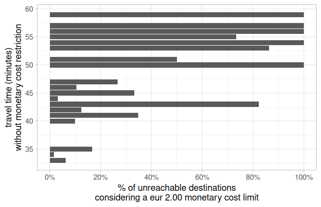
# plot of unreachable destinations when the monetary cost limit is too low
unreachable <- ttm %>%
  group_by(travel_time_unl, missing = is.na(travel_time_200)) %>%
  summarise(count = n(), .groups = "drop_last") %>%   # keep grouping by travel_time_unl
  mutate(perc = count / sum(count, na.rm = TRUE)) %>%
  ungroup() %>%
  filter(missing) %>%          # keep only rows where travel_time_200 was NA
  tidyr::drop_na()

p2 <- ggplot(unreachable, aes(x=travel_time_unl, y=perc)) +
  geom_col() +
  coord_flip() +
  scale_x_continuous(breaks = seq(0, 60, 5)) +
  scale_y_continuous(limits = c(0, 1), breaks = seq(0, 1, 0.2), 
                     labels = paste0(seq(0, 100, 20), "%")) +
  theme_light() +
  labs(x = "travel time (minutes)\nwithout monetary cost restriction",
       y = "% of unreachable destinations\nconsidering a eur 2.00 monetary cost limit")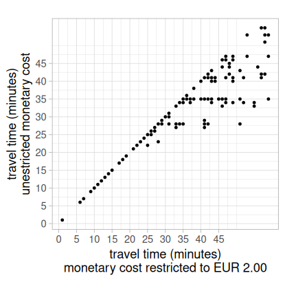

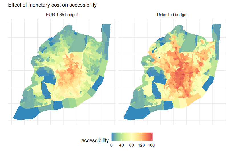
Calculating accessibility with monetary cost

To Healthcare facilities

GRID_data = readRDS("data/Lisbon/GRIDhex_data.rds")
GRID_df = GRID_data |> st_drop_geometry()

# calculate accessibility function
calculate_accessibility <- function(fare, fare_string) {
  access_df <- accessibility(
    r5r_lisboa,
    origins = GRID_df,
    destinations = GRID_df,
    mode = c("WALK", "TRANSIT"),
    departure_datetime = departure_datetime,
    time_window = 1,
    opportunities_colname = "healthcare",
    cutoffs = 40,
    fare_structure = fare_structure,
    max_fare = fare,
    max_trip_duration = 60,
    max_walk_time = 15,
    progress = FALSE)

  access_df$max_fare <- fare_string

  return(access_df)
}

# calculate accessibility, combine results, and convert to SF
access_165 <- calculate_accessibility(fare=1.65, fare_string="EUR 1.65 budget")
access_unl <- calculate_accessibility(fare=Inf, fare_string="Unlimited budget")

access <- rbind(access_165, access_unl)

# bring geometry
access = access |> 
  left_join(GRID_df |>
              select(id, h3_address) |>
              mutate(id = as.character(id)))
access$geometry = h3jsr::cell_to_polygon(access$h3_address)
access <- st_as_sf(access)

Code

# plot accessibility maps
ggplot(data = access) +
  geom_sf(aes(fill = accessibility), color=NA, size = 0.2) +
  scale_fill_distiller(palette = "Spectral") +
  facet_wrap(~max_fare) +
  labs(subtitle = "Effect of monetary cost on accessibility") +
  theme_minimal() +
  theme(legend.position = "bottom",
        axis.text = element_blank())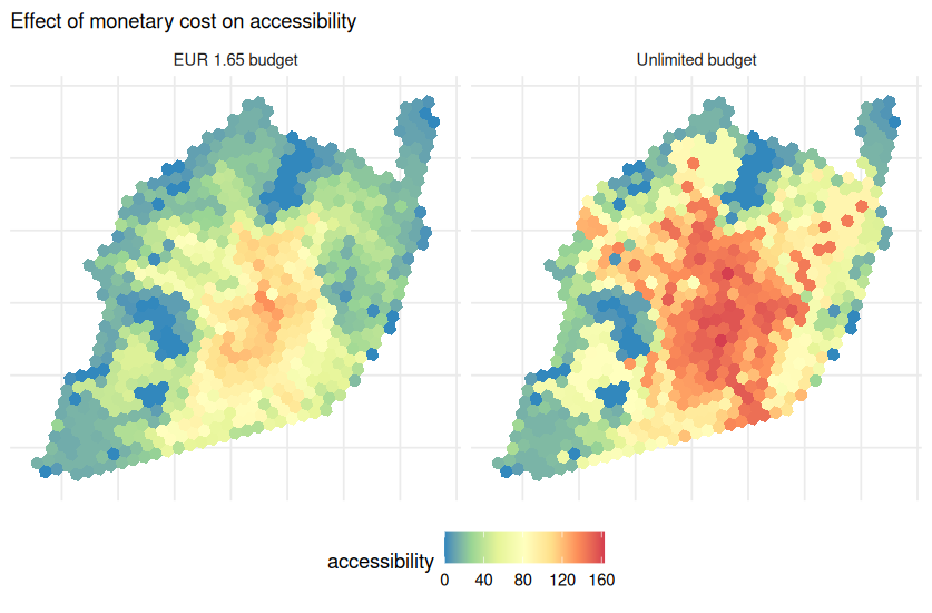

Reading suggestion

The impact of transit monetary costs on transport inequality (Herszenhut et al. 2022)

The cost of equity: Assessing transit accessibility and social disparity using total travel cost (El-Geneidy et al. 2016)

References

El-Geneidy, Ahmed, David Levinson, Ehab Diab, Genevieve Boisjoly, David Verbich, and Charis Loong. 2016. “The Cost of Equity: Assessing Transit Accessibility and Social Disparity Using Total Travel Cost.” Transportation Research Part A: Policy and Practice 91 (September): 302–16. https://doi.org/10.1016/j.tra.2016.07.003.

Herszenhut, Daniel, Rafael H. M. Pereira, Licinio da Silva Portugal, and Matheus Henrique de Sousa Oliveira. 2022. “The Impact of Transit Monetary Costs on Transport Inequality.” Journal of Transport Geography 99 (February): 103309. https://doi.org/10.1016/j.jtrangeo.2022.103309.

Pereira, Rafael H. M., Marcus Saraiva, Daniel Herszenhut, Carlos Kaue Vieira Braga, and Matthew Wigginton Conway. 2021. “R5r: Rapid Realistic Routing on Multimodal Transport Networks with r ⁵ in r.” Findings, March. https://doi.org/10.32866/001c.21262.

Create rules for an operator

Calculating a pareto_frontier()

Calculating accessibility with monetary cost

References

Calculating a `pareto_frontier()`