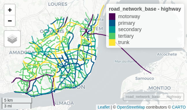
# load osm export in .gpkg
road_network = sf::st_read("data/Lisbon/Lisbon_road_network.gpkg", quiet = TRUE)

# filter main roads
road_network_base = road_network |>
  filter(highway %in% c("primary", "secondary", "tertiary", "trunk", "motorway")) |>
  select(osm_id, name, highway)

# map
mapview::mapview(road_network_base, zcol = "highway")Network setup
In this chapter we will guide you through the data requirements, data collection, and setting up a multi-modal network with r5r.
Tip
You should start an R script with all the data preparation, such as data_prep.R
Data requirements
You will need R and r5r (Pereira et al. 2021) package installed on your computer.
r5r sets-up a network file .dat by combining the following datasets in the same folder:
- Road Network (OpenStreetMap1 as
.osm.pbf) - GTFS2 from PTransit operators (a single
.zipor several) - Digital Elevation Model3 (
.tif), to consider impedances for walking and cycling
For the documentation of data needed, see r5r::build_network
Road Networks
OpenStreetMap
The OpenStreetMap is a collaborative online mapping project that creates a free editable map of the world.
This is the most used source of road network data for transportation analysis in academia, since it is available almost everywhere in the world, is open and free to use.
Although it can be not 100% accurate, OSM is a good source of data for most of the cases.
You can access it’s visualization tool at www.openstreetmap.org. To edit the map, you can use the Editor, once you register.
If you want to download the data, you can use the following tools.
These websites include all the OSM data, with much more information than you need.
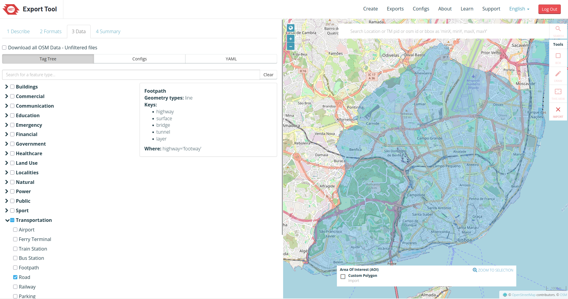
HOT Export Tool
This interactive tool helps you to select the region you want to extract (or import an existing city_limit.geojson4), the type of information to include, and the output data format.
Access via export.hotosm.org5. Select format as .gpkg and .pbf.
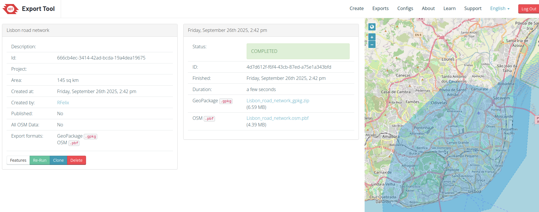
After the export, you can read in R using the sf package:
OSM in R
There are also some R packages that can help you to download and work with OpenStreetMap data, such as:
This is an example of how to download OpenStreetMap road network data using the osmextract package:
library(osmextract)
OSM_Malta = oe_get_network(place = "Malta") # it will geocode the place

Malta_main_roads = OSM_Malta |>
  filter(highway %in% c("primary", "secondary", "tertiary", "trunk"))

plot(Malta_main_roads["highway"])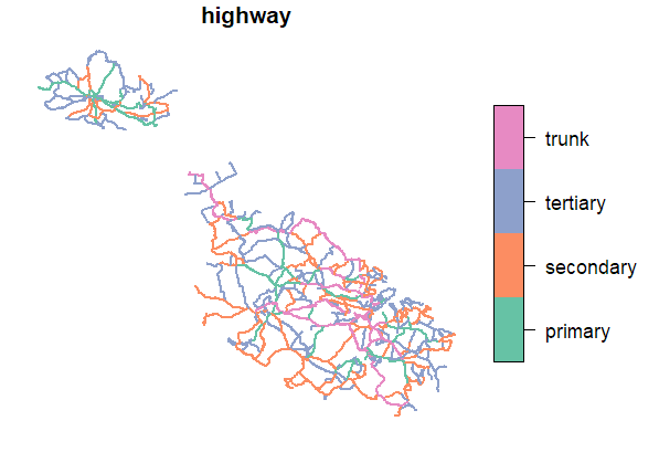
GTFS - Transportation Services’ Data
General Transit Feed Specification (GTFS) is standard format for documenting public transportation information, including: routes, schedules, stop locations, calendar patterns, trips, and possible transfers. Transit agencies are responsible for maintaining the data up-to-date.
This information is used in several applications, such as Google Maps, to provide public transportation directions. It can be offered for a city, a region, or even a whole country, depending on the PT agency.
The recent version 2 of the GTFS standard includes more information, such as real-time data.
The data is usually in a .zip file that includes several .txt files (one for each type of information) with tabular relations.
Online sources
You can find most GTFS data in the following websites:
Some PT agencies also provide their open-data in their websites.
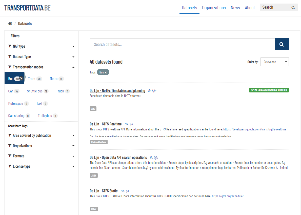
National Access Points
The European Union has a directive that requires the member states to provide access to transportation data. Data includes not only Public Transportation data, but also road networks, car parking, and other transportation-related information.
List of the European Union members states with National Access Points for Transportation data
Example of Bus services data in Belgium:
R packages
There are some nice R packages to read and manipulate GTFS data, such as:
Be aware that they may share the same function names, so it is important to use of of them at the time.
Create shapes.txt
Some operators do not include the information, because this is not a mandatory file.
Anyway, you can create this file with some GIS operations, simplified by GTFSwizard::read_gtfs()
GTFSwizard::get_shapes reconstructs the shapes table using euclidean approximation, based on the coordinates and sequence of stops for each trip, and may not be accurate.
Install GTFSwizard
remotes::install_github("hrbrmstr/hrbrthemes") # in 10.2025 this dependency was missing
remotes::install_github('OPATP/GTFSwizard@main')
If your zip contains shapes.txt that exist but are empty, delete that file before proceeding.
library(GTFSwizard)
gtfs_noshapes = read_gtfs("original/gtfs_without_shapes.zip") # it will recrreate shapes
summary(gtfs_noshapes)
write_gtfs(gtfs_noshapes, "data/r5r/gtfs_with_shapes.zip") # save the result
Sometimes, event this will not work because other information is missing in the .zip
Consider searching for another data source, or changing to another city.
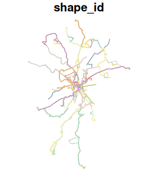
Filter GTFS by area
Having a very large GTFS, as a nation-wide, instead of a city-wide one, can hold too much information not required. You may want to crop it by using tidytransit::filter_feed_by_area()
This probably does not affect your r5r network model, anyway.
# example with Gent, Belgium
area = st_read("data/gent.geojson") # city_limit

# load gtfs
gtfs_large = tidytransit::read_gtfs("https://data.gtfs.be/delijn/gtfs/be-delijn-gtfs.zip") # direct link

# filter by area
gtfs_crop = tidytransit::filter_feed_by_area(gtfs_large, area)

# get shapes
gtfs_large_shapes = shapes_as_sf(gtfs_large$shapes)
gtfs_crop_shapes = shapes_as_sf(gtfs_crop$shapes)

# compare
plot(gtfs_large_shapes)
plot(gtfs_crop_shapes)

write_gtfs(gtfs_crop, "data/r5r/gent_redux.zip") # save for modelling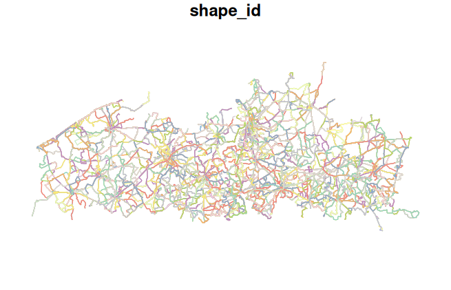
Create transfers.txt
Some operators do not include the information regarding where can someone change from bus A to bus B, because this is not a mandatory file.
Anyway, you can create this file with some GIS operations, simplified by gtfsrouter::gtfs_transfer_table()
# Donwload and save zip
carris_url = "https://gateway.carris.pt/gateway/gtfs/api/v2.8/GTFS" # direct link
download.file(carris_url, destfile = "original/carris_gtfs.zip")

carris_notransfers = gtfsrouter::extract_gtfs("original/carris_gtfs.zip")
carris_transfers = gtfsrouter::gtfs_transfer_table(carris_notransfers)
write.csv(carris_transfers[["transfers"]], "original/transfers.txt", row.names = F, quote = F)
# drag and drop this transfers.txt file into the zip file

carris = tidytransit::read_gtfs("original/carris_gtfs.zip")
tidytransit::validate_gtfs(carris) # validate
Merge GTFS sources
Public transit analysis takes advantage of the standardized GTFS format. However, its provision by operator makes it difficult for network aggregated analysis, considering connectivity and multimodality. GTFShift::unify() proposes a simple solution to this problem, generating an aggregated GTFS file given several instances of these.
The unification produces a single GTFS instance, saved as a ZIP file. Option create_transfers enables the generation of transfers.txt, aggregating close stops, even if from different GTFS.
gtfs_united = GTFShift::unify(gtfs_1, gtfs_2, create_transfers = TRUE)
write_gtfs(gtfs_united, "data/r5r/gtfs_united.zip") # save for modelling
Elevation
This information is useful if your city is somehow hilly, and you are modelling pedestrian and/or bike travel.
In the following websites you can export a raster file of Digital Elevation Model (DEM) in .tif format:
- elevatr R package
- Nasa’s SRTMGL1 website
- Copernicus EU website
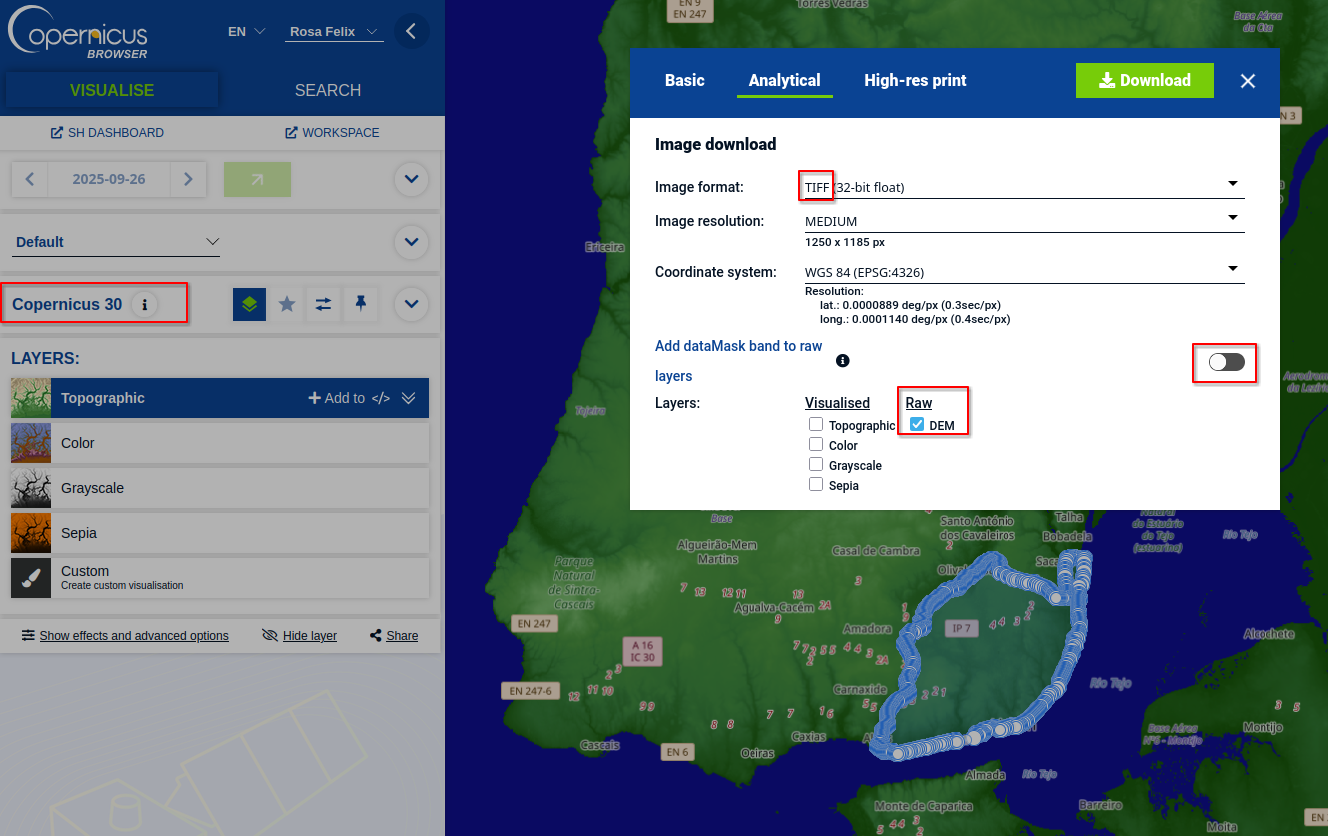
The dem should be renamed to .tif (single F) instead of .tiff, otherwise it will be ignored in r5r build.
Verify in R
dem = terra::rast("data/Lisbon/Copernicus_30m.tif") # rename the extension to .tif !!
terra::plot(dem)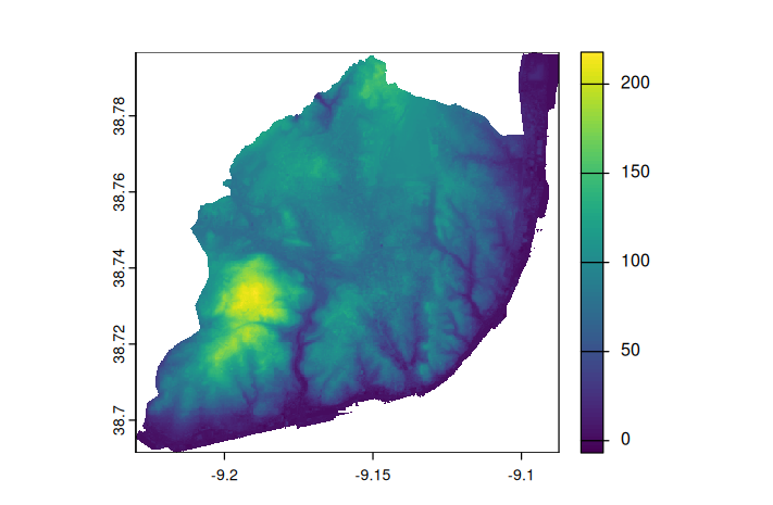
Setting up a routable transport network
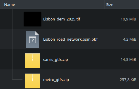
Your folder should contain these files, such as:
# Load packages
library(tidyverse)
library(sf)
options(java.parameters = '-Xmx8G') # allocate memory for 8GB
library(r5r)data_path= "data/Lisbon/r5r" # relative path to your folder containing the required data
network = build_network(
data_path,
elevation = "TOBLER" # optional. MINETTI or NONE
)If you already have a network.dat file, it will use that pre-build network.
Check if your transportation network is correct:
transit_net = transit_network_to_sf(r5r_lisboa)
mapview::mapview(transit_net$routes, zcol = "mode")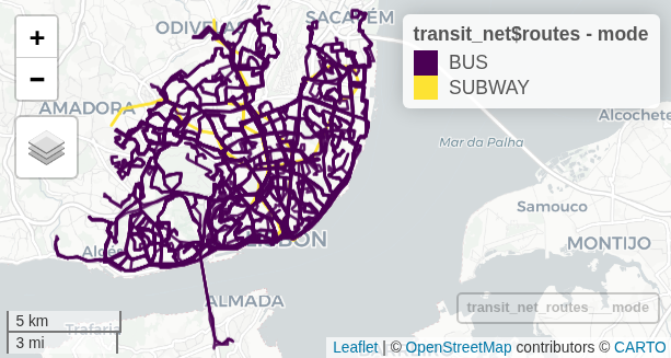
References
Pereira, Rafael H. M., Marcus Saraiva, Daniel Herszenhut, Carlos Kaue Vieira Braga, and Matthew Wigginton Conway. 2021. “R5r: Rapid Realistic Routing on Multimodal Transport Networks with r ⁵ in r.” Findings, March. https://doi.org/10.32866/001c.21262.
Footnotes
See how to export an area with HOT export tool.↩︎
Optional.↩︎
Optional.↩︎
For instance, see here for Germany: https://opendatalab.de/projects/geojson-utilities/↩︎
You need an OSM account to use it.↩︎