6  Multiple Linear Regression

Do it yourself with R

Copy the script MultipleLinarRegression.R and paste it in your session.
Run each line using CTRL + ENTER

Your task

Estimate a linear regression model that predicts the car percentage per district.

6.1 Load packages

library(tidyverse) # Pack of most used libraries for data science
library(skimr) # summary of the data
library(DataExplorer) # exploratory data analysis
library(corrplot) # correlation plots

library(car) # Testing autocorrelation (Durbin Watson)
library(olsrr) # Testing multicollinearity (VIF, TOL, etc.)

6.2 Dataset

The database used in this example is a treated database from the Mobility Survey for the metropolitan areas of Lisbon in 2018 (INE 2018).

Included variables:

• Origin_dicofre16 - Code of Freguesia (district) as set by INE after 2016 (Distrito + Concelho + Freguesia), for trip origin
• Total - number of trips with origin at each district
• Walk - number of walking trips
• Bike - number of bike trips
• Car - number of car trips. Includes taxi and motorcycle.
• PTransit - number of Public Transit trips
• Other - number of other trips (truck, van, tractor, aviation)
• Distance - average trip distance (km)
• Duration - average trip duration (minutes)
• Car_perc - percentage of car trips
• N_INDIVIDUOS - number of residents (INE 2022)
• Male_perc - percentage of male residents (INE 2022)
• IncomeHH - average household income
• Nvehicles - average number of car/motorcycle vehicles in the household
• DrivingLic - percentage of car driving licence holders
• CarParkFree_Work - percentage of respondents with free car parking at the work location
• PTpass - percentage of public transit monthly pass holders
• internal - binary variable (factor). Yes: trip with same TAZ origin and destination, No: trips with different destination
• Lisboa - binary variable (factor). Yes: the district is part of Lisbon municipality, No: otherwise
• Area_km2 - area of in Origin_dicofre16, in km²

Import dataset

data = readRDS("../data/IMOBmodel.Rds")
data_continuous = data |> select(-Origin_dicofre16, -internal, -Lisboa) # Exclude categorical variables

Show summary statistics

skim(data)

Data summary

Name	data
Number of rows	236
Number of columns	20
_______________________
Column type frequency:
character	1
factor	2
numeric	17
________________________
Group variables	None

Variable type: character

skim_variable	n_missing	complete_rate	min	max	empty	n_unique	whitespace
Origin_dicofre16	0	1	6	6	0	118	0

Variable type: factor

skim_variable	n_missing	complete_rate	ordered	n_unique	top_counts
internal	0	1	FALSE	2	Yes: 118, No: 118
Lisboa	0	1	FALSE	2	No: 188, Yes: 48

Variable type: numeric

skim_variable	n_missing	complete_rate	mean	sd	p0	p25	p50	p75	p100	hist
Total	0	1	22457.00	19084.45	361.00	5917.75	17474.00	33377.50	112186.00	▇▃▂▁▁
Walk	0	1	5383.44	6224.84	0.00	763.25	3125.00	8298.50	32646.00	▇▂▁▁▁
Bike	0	1	107.03	248.65	0.00	0.00	13.50	98.75	2040.00	▇▁▁▁▁
Car	0	1	13289.24	12351.61	0.00	3243.00	9008.00	21248.75	52631.00	▇▃▂▁▁
PTransit	0	1	3473.79	5467.82	0.00	249.00	1057.00	4853.00	41672.00	▇▁▁▁▁
Other	0	1	203.45	336.04	0.00	2.00	44.00	281.50	2391.00	▇▁▁▁▁
Distance	0	1	11.14	2.66	6.84	9.54	10.32	12.10	22.66	▇▇▂▁▁
Duration	0	1	25.42	3.91	16.30	23.00	24.70	27.73	37.42	▁▇▆▂▁
Car_perc	0	1	59.00	21.56	0.00	45.40	62.62	75.72	99.27	▁▃▆▇▅
N_INDIVIDUOS	0	1	24323.80	16438.04	1566.00	11060.00	20855.00	36079.00	68649.00	▇▆▅▃▁
Male_perc	0	1	47.54	1.57	44.61	46.58	47.50	48.29	55.94	▅▇▂▁▁
IncomeHH	0	1	1732.55	453.11	884.46	1417.76	1594.73	1953.50	3462.32	▃▇▃▁▁
Nvehicles	0	1	1.53	0.24	1.02	1.35	1.54	1.67	2.42	▃▇▆▂▁
DrivingLic	0	1	62.50	8.12	37.04	57.67	63.00	68.84	80.79	▁▂▇▇▂
CarParkFree_Work	0	1	49.30	14.30	5.47	40.39	50.51	57.92	87.60	▁▃▇▇▁
PTpass	0	1	23.82	12.87	0.00	13.41	22.72	32.94	60.45	▅▇▇▂▁
Area_km2	0	1	25.55	42.58	1.49	5.04	11.60	28.51	282.13	▇▁▁▁▁

The dependent variable is continuous.

6.3 Check the assumptions

Before running the model, you need to check if the assumptions are met.

1. The dependent variable is normally distributed
2. Linear relationship between the dependent variable and the independent variables
3. No multicollinearity between independent variables (or only very little)
4. The observations are independent
5. Constant Variance (Assumption of Homoscedasticity)
6. Residuals are normally distributed

6.4 Assumption 1: Normal distribution

The Dependent Variable is be normally distributed.

Check the histogram of Car_perc:

hist(data$Car_perc)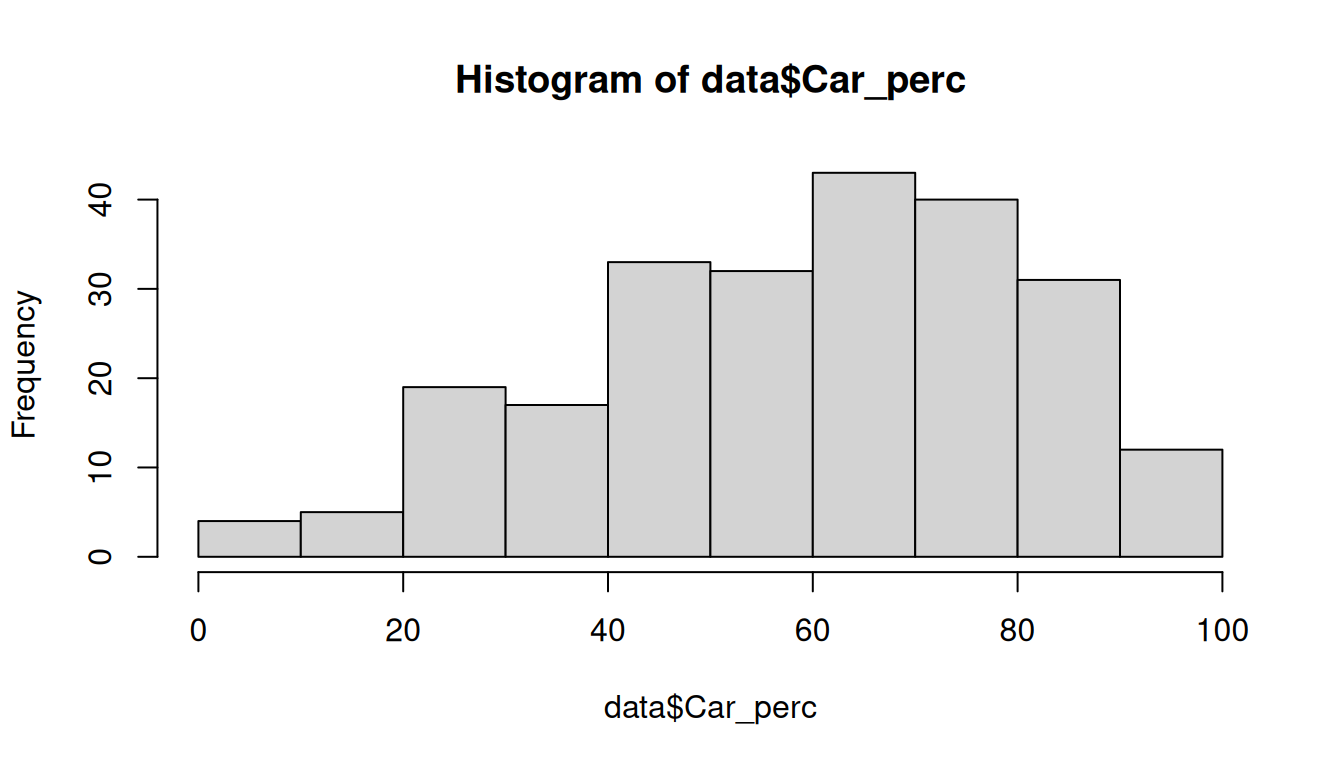

If the sample is small (< 50 observations), we use Shapiro-Wilk test:

shapiro.test(data$Car_perc)

    Shapiro-Wilk normality test

data:  data$Car_perc
W = 0.97284, p-value = 0.0001709

If not, use the Kolmogorov-Smirnov test:

ks.test(
  data$Car_perc,
  "pnorm",
  mean = mean(data$Car_perc),
  sd = sd(data$Car_perc)
)

    Asymptotic one-sample Kolmogorov-Smirnov test

data:  data$Car_perc
D = 0.072477, p-value = 0.1675
alternative hypothesis: two-sided

The null hypothesis for both tests is that the distribution is normal. Therefore, for the distribution to be normal, the pvalue must be > 0.05 and the null hypothesis is not rejected. From the output obtained we can assume normality.

6.5 Assumption 2: Linear relationship

There is a linear relationship between dependent variable (DV) and independent variables (IV).

We can check this assumption by plotting scatterplots of the DV against each IV:

plot(x = data$Car_perc, y = data$Total, xlab = "Car_perc (%)", ylab = "Total (number of trips)")  
plot(x = data$Car_perc, y = data$Walk, xlab = "Car_perc", ylab = "Walk")  
plot(x = data$Car_perc, y = data$Bike, xlab = "Car_perc", ylab = "Bike")  
plot(x = data$Car_perc, y = data$Car, xlab = "Car_perc", ylab = "Car")  
plot(x = data$Car_perc, y = data$PTransit, xlab = "Car_perc", ylab = "PTransit")
plot(x = data$Car_perc, y = data$Other, xlab = "Car_perc", ylab = "Other")
plot(x = data$Car_perc, y = data$Distance, xlab = "Car_perc", ylab = "Distance")
plot(x = data$Car_perc, y = data$Duration, xlab = "Car_perc", ylab = "Duration")
plot(x = data$Car_perc, y = data$N_INDIVIDUOS, xlab = "Car_perc", ylab = "N_INDIVIDUOS")
plot(x = data$Car_perc, y = data$Male_perc, xlab = "Car_perc", ylab = "Male_perc")
plot(x = data$Car_perc, y = data$IncomeHH, xlab = "Car_perc", ylab = "IncomeHH")
plot(x = data$Car_perc, y = data$Nvehicles, xlab = "Car_perc", ylab = "Nvehicles")
plot(x = data$Car_perc, y = data$DrivingLic, xlab = "Car_perc", ylab = "Driving License")
plot(x = data$Car_perc, y = data$CarParkFree_Work, xlab = "Car_perc", ylab = "Free car parking at work")
plot(x = data$Car_perc, y = data$PTpass, xlab = "Car_perc", ylab = "PTpass")
plot(x = data$Car_perc, y = data$internal, xlab = "Car_perc", ylab = "internal trips")
plot(x = data$Car_perc, y = data$Lisboa, xlab = "Car_perc", ylab = "Lisboa")
plot(x = data$Car_perc, y = data$Area_km2, xlab = "Car_perc", ylab = "Area_km2")

Or you can make a pairwise scatterplot matrix, that compares every variable with each other:

# pairs(data_continuous, pch = 19, lower.panel = NULL) # we have too many variables, let's split the plots
pairs(data_continuous[,1:6], pch = 19, lower.panel = NULL)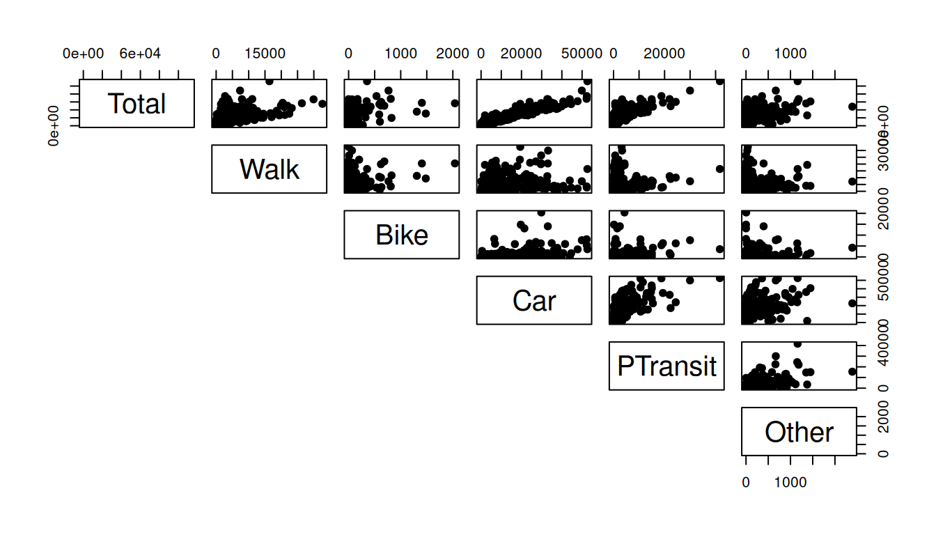

pairs(data_continuous[,7:12], pch = 19, lower.panel = NULL)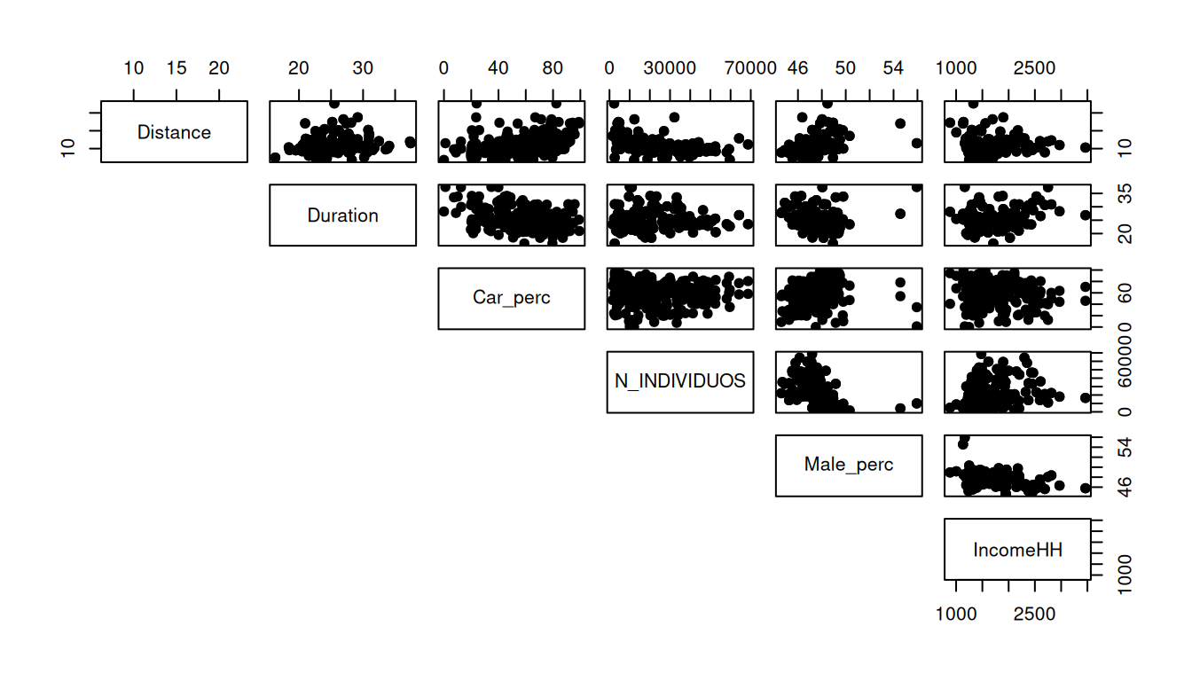

pairs(data_continuous[,13:17], pch = 19, lower.panel = NULL)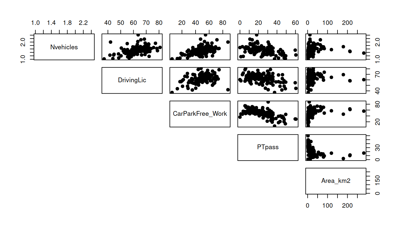

6.6 Assumption 3: No multicollinearity

Check the correlation plot before choosing the variables.

Declare the model

Use CTRL + SHIFT + C to comment/uncomment lines (variables)

# names(data) # to see the names of the variables

model = lm(
  Car_perc ~
    Total +
    Walk +
    Bike +
    Car +
    PTransit +
    Other +
    Distance + 
    Duration + 
    N_INDIVIDUOS + 
    Male_perc + 
    IncomeHH + 
    Nvehicles + 
    DrivingLic + 
    CarParkFree_Work + 
    PTpass + 
    internal + 
    Lisboa + 
    Area_km2,
  data = data
)

summary(model)

Call:
lm(formula = Car_perc ~ Total + Walk + Bike + Car + PTransit + 
    Other + Distance + Duration + N_INDIVIDUOS + Male_perc + 
    IncomeHH + Nvehicles + DrivingLic + CarParkFree_Work + PTpass + 
    internal + Lisboa + Area_km2, data = data)

Residuals:
    Min      1Q  Median      3Q     Max 
-37.952  -4.907  -0.232   5.305  39.157 

Coefficients:
                   Estimate Std. Error t value Pr(>|t|)    
(Intercept)       4.047e+00  3.192e+01   0.127  0.89923    
Total             1.633e-01  3.671e-01   0.445  0.65700    
Walk             -1.640e-01  3.671e-01  -0.447  0.65552    
Bike             -1.614e-01  3.669e-01  -0.440  0.66044    
Car              -1.627e-01  3.671e-01  -0.443  0.65806    
PTransit         -1.640e-01  3.672e-01  -0.447  0.65552    
Other            -1.622e-01  3.671e-01  -0.442  0.65897    
Distance          6.004e-01  3.629e-01   1.654  0.09948 .  
Duration         -3.244e-01  3.325e-01  -0.976  0.33032    
N_INDIVIDUOS     -6.627e-05  8.876e-05  -0.747  0.45612    
Male_perc         2.723e-01  6.151e-01   0.443  0.65849    
IncomeHH         -5.218e-04  2.199e-03  -0.237  0.81264    
Nvehicles         7.301e+00  3.959e+00   1.844  0.06650 .  
DrivingLic        2.910e-01  1.161e-01   2.506  0.01294 *  
CarParkFree_Work  1.943e-01  7.882e-02   2.465  0.01449 *  
PTpass           -8.254e-02  9.989e-02  -0.826  0.40956    
internalNo        1.962e+01  2.136e+00   9.182  < 2e-16 ***
LisboaYes        -9.647e+00  3.182e+00  -3.031  0.00273 ** 
Area_km2          1.689e-02  1.860e-02   0.908  0.36486    
---
Signif. codes:  0 '***' 0.001 '**' 0.01 '*' 0.05 '.' 0.1 ' ' 1

Residual standard error: 10.59 on 217 degrees of freedom
Multiple R-squared:  0.7772,    Adjusted R-squared:  0.7587 
F-statistic: 42.06 on 18 and 217 DF,  p-value: < 2.2e-16

Assessing the model

1. First check the pvalue and the F statistics of the model to see if there is any statistical relation between the dependent variable and the independent variables. If pvalue < 0.05 and the F statistics > Fcritical = 2.39, then the model is statistically acceptable.

2. The R-square and Adjusted R-square evaluate the amount of variance that is explained by the model. The difference between one and another is that the R-square does not consider the number of variables. If you increase the number of variables in the model, the R-square will tend to increase which can lead to overfitting. On the other hand, the Adjusted R-square adjust to the number of independent variables.

3. Take a look at the t-value and the Pr(>|t|). If the t-value > 1.96 or Pr(>|t|) < 0.05, then the IV is statistically significant to the model.

4. To analyse the estimates of the variables, you should first check the signal and assess if the independent variable has a direct or inverse relationship with the dependent variable. It is only possible to evaluate the magnitude of the estimate if all variables are continuous and standardized or by calculating the elasticities. Do not forget to access the Intercept…

We can see from the output that the R-squared value for the model (with ALL variables) is 0.7772. We can also see that the overall F-statistic is 42.06 and the corresponding p-value is <2.2e-16, which indicates that the overall regression model is significant. Also, the predictor variables DrivingLic and CarParkFree_Work, internal(No) and Lisboa(Yes) are statistically significant at the 0.05 significance level.

Your turn

Now try to remove some variables from the model and assess it again. Elaborate a justification to exclude those variables.

Calculate the Variance Inflation Factor (VIF)

We use the vif() function from the car package to calculate the VIF for each predictor variable in the model:

car::vif(model)

           Total             Walk             Bike              Car 
    1.028324e+08     1.094004e+07     1.743544e+04     4.307486e+07 
        PTransit            Other         Distance         Duration 
    8.443136e+06     3.186972e+04     1.957062e+00     3.544018e+00 
    N_INDIVIDUOS        Male_perc         IncomeHH        Nvehicles 
    4.459671e+00     1.961472e+00     2.079348e+00     1.882275e+00 
      DrivingLic CarParkFree_Work           PTpass         internal 
    1.863227e+00     2.660375e+00     3.464699e+00     2.400178e+00 
          Lisboa         Area_km2 
    3.451852e+00     1.313708e+00 

A common rule of thumb is that a VIF value greater than 5 indicates a high level of multicollinearity among the predictor variables, which is potentially concerning.

Condition index

Condition index is another diagnostic tool for detecting multicollinearity, with values above 10 indicating moderate multicollinearity and values above 30 indicating severe multicollinearity. You will learn how to to that in the next class: Factor analysis.

6.7 Assumption 4: Independence of observations

Multiple linear regression assumes that each observation in the dataset is independent.

The error (E) is independent across observations and the error variance is constant across IV

The simplest way to determine if this assumption is met is to perform a Durbin-Watson test, which is a formal statistical test that tells us whether or not the residuals (and thus the observations) exhibit autocorrelation.

durbinWatsonTest(model)

 lag Autocorrelation D-W Statistic p-value
   1      0.07881007      1.840798   0.104
 Alternative hypothesis: rho != 0

Note

In the Durbin-Watson test, values of the D-W Statistic vary from 0 to 4.

If the values are from 1.8 to 2.2 this means that there is no autocorrelation in the model.

H₀ (null hypothesis): There is no correlation among the residuals. Since p-value > 0.05, we do not reject the null hypothesis and we can not discard that there is autocorrelation in the model.

If the observations are not independent, you may consider to treat the observarions as a panel data.

6.8 Assumption 5: Constant Variance (Homoscedasticity)

The simplest way to determine if this assumption is met is to create a plot of standardized residuals versus predicted values.

plot(model)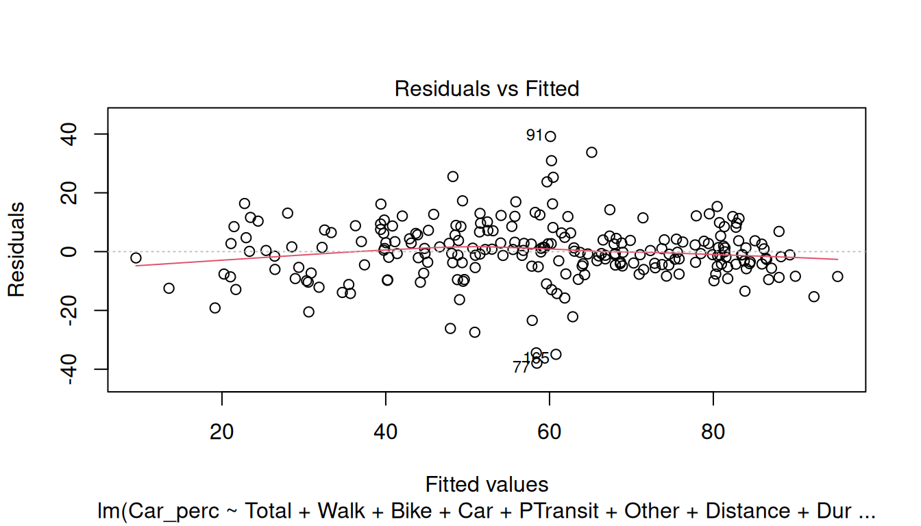

For the Residuals, check the following assumptions:

• Residuals vs Fitted: This plot is used to detect non-linearity, heteroscedasticity, and outliers.

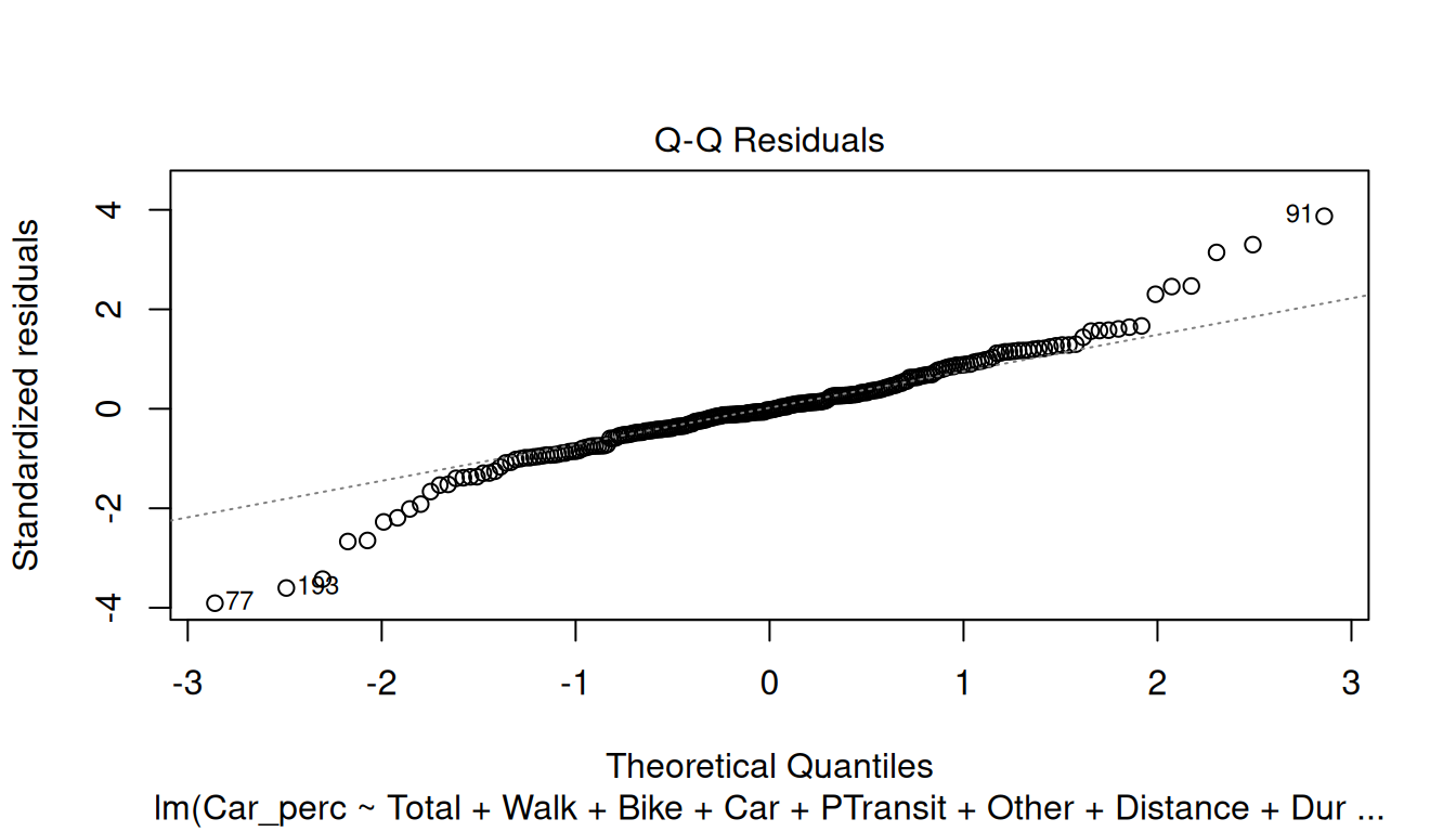
• Normal Q-Q: The quantile-quantile (Q-Q) plot is used to check if the disturbances follow a normal distribution

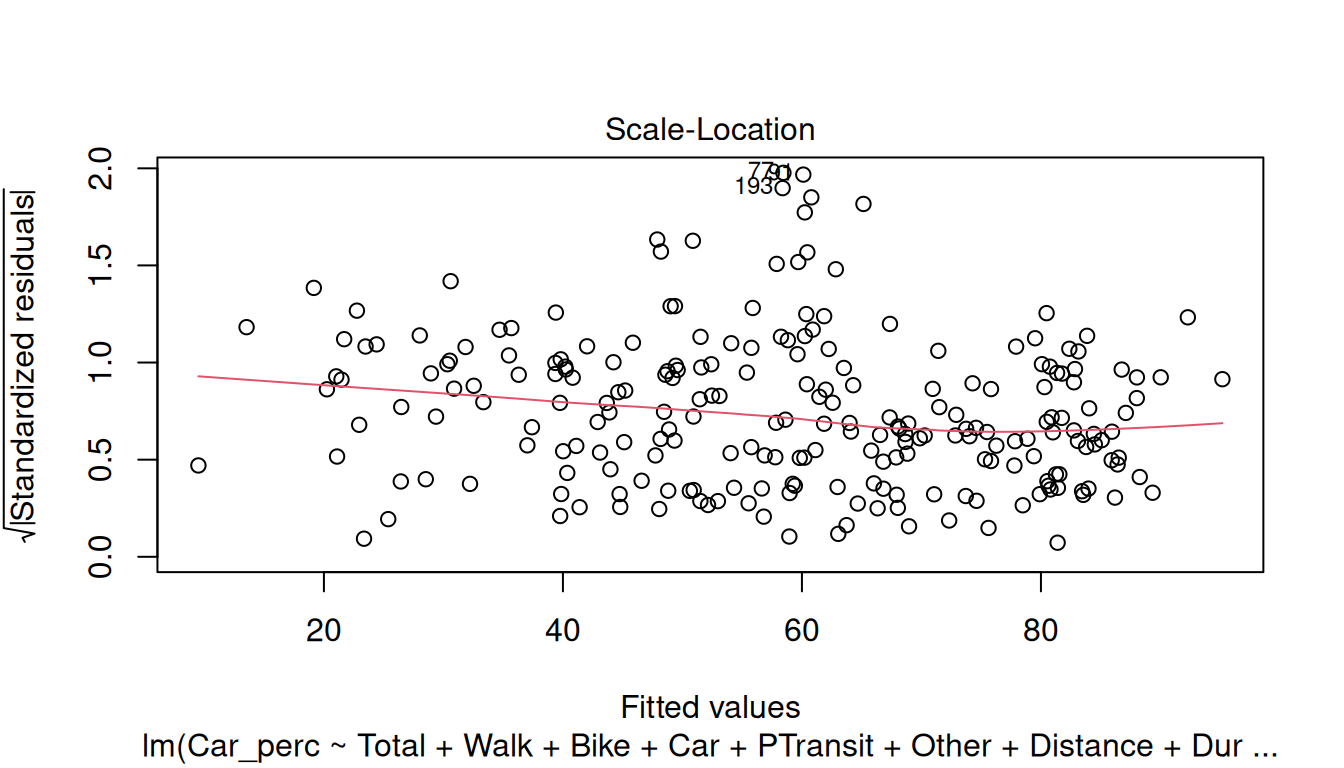
• Scale-Location: This plot is used to verify if the residuals are spread equally (homoscedasticity) or not (heteroscedasticity) through the sample.

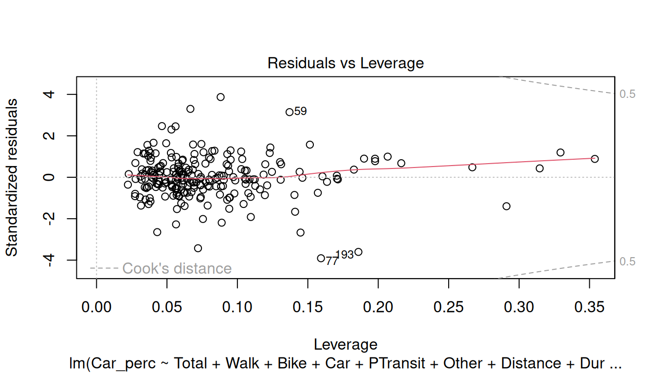
• Residuals vs Leverage: This plot is used to detect the impact of the outliers in the model. If the outliers are outside the Cook-distance, this may lead to serious problems in the model.

Try analyzing the plots and check if the model meets the assumptions.

6.9 Assumption 6: Residuals are normally distributed

Assess the Q-Q Residuals plot above. When the residuals clearly depart from a straight diagonal line, it indicates that they do not follow a normal distribution.

Use a formal statistical test like Shapiro-Wilk or Kolmogorov-Smironov to validate those results.

INE. 2018. “Mobilidade e Funcionalidade Do Território Nas Áreas Metropolitanas do Porto e de Lisboa: 2017.” Lisboa: Instituto National de Estatística. https://www.ine.pt/xportal/xmain?xpid=INE&xpgid=ine_publicacoes&PUBLICACOESpub_boui=349495406&PUBLICACOESmodo=2&xlang=pt.

———. 2022. “Censos 2021- XVI Recenseamento Geral da População. VI Recenseamento Geral da Habitação.” Lisboa: Instituto National de Estatística. https://censos.ine.pt/xurl/pub/65586079.