Introduction
Data classification helps to categorize transit data into meaningful
groups based on specific criteria or thresholds. This process is
essential for interpreting complex datasets, enabling transit planners
and analysts to make informed decisions regarding service improvements,
resource allocation, and policy development. GTFShift
provides methods that encapsulate methodologies for this purpose. This
document explores their applicability with simple examples.
This article uses a GTFS feed from the library GTFS database for Portugal as an example. Refer to the vignette(“download”) for more details.
# Get GTFS from library GTFS database for Portugal
data = read.csv(system.file("extdata", "gtfs_sources_pt.csv", package = "GTFShift"))
gtfs_id = "barreiro"
gtfs = GTFShift::load_feed(data$URL[data$ID == gtfs_id], create_transfers=FALSE)
Bus frequency LOS
Bus frequency level of service (LOS) classification is a methodology
used to evaluate the quality of bus services based on their frequency.
The classification is based on the Highway Capacity Manual (HCM) 2000
guidelines on “Service Frequency LOS for Urban Scheduled Transit
Service” (Exhibit 27-1), implemented in
GTFShift::classify_frequency_los().
The LOS categories range from A to F, with A representing the highest level of service (most frequent buses) and F representing the lowest level of service (least frequent buses).
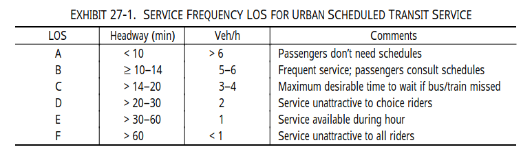
Note that this method is an adaptation of the original method, as it originally classifies LOS based on headway (time) and not frequency (number of buses per hour), being this last one a proxy.
Also, mind that HCM states that “LOS is determined by destination from a given transit stop, since several routes may serve a given stop but not all may serve a particular destination”. Applications of this method to other scenarios should consider this aspect.
# Get route frequency analysis
frequency_analysis = GTFShift::get_route_frequency_hourly(gtfs)

# Classify frequency level of service
frequency_los = GTFShift::classify_frequency_los(frequency_analysis)

frequency_los
#> Simple feature collection with 425 features and 7 fields
#> Geometry type: LINESTRING
#> Dimension:     XY
#> Bounding box:  xmin: -9.084467 ymin: 38.57161 xmax: -9.01185 ymax: 38.67369
#> Geodetic CRS:  WGS 84
#> # A tibble: 425 × 8
#>    route_id       shape_id    route_short_name direction_id  hour frequency
#>  * <chr>          <chr>       <chr>                   <int> <int>     <int>
#>  1 10_10-COINA-FT 10-COINA-FT 10                          0     7         1
#>  2 10_10-COINA-FT 10-COINA-FT 10                          0     8         1
#>  3 10_10-COINA-FT 10-COINA-FT 10                          0     9         2
#>  4 10_10-COINA-FT 10-COINA-FT 10                          0    10         1
#>  5 10_10-COINA-FT 10-COINA-FT 10                          0    11         1
#>  6 10_10-COINA-FT 10-COINA-FT 10                          0    12         2
#>  7 10_10-COINA-FT 10-COINA-FT 10                          0    13         1
#>  8 10_10-COINA-FT 10-COINA-FT 10                          0    14         2
#>  9 10_10-COINA-FT 10-COINA-FT 10                          0    15         1
#> 10 10_10-COINA-FT 10-COINA-FT 10                          0    16         2
#> # ℹ 415 more rows
#> # ℹ 2 more variables: geometry <LINESTRING [°]>, frequency_los <chr>

table(frequency_los$frequency_los)
#>
#>   A   B   C   D   E
#>   3  25  89 110 198