Introduction
Analyzing public transit feeds is important to understand its
territorial coverage and dynamics, both on its spatial and temporal
dimensions. GTFShift provides several methods that
encapsulate pre-defined methodologies for them. This document explores
their applicability with simple examples.
This article uses a GTFS feed from the library GTFS database for Portugal as an example. Refer to the vignette(“download”) for more details.
# Get GTFS from library GTFS database for Portugal
data = read.csv(system.file("extdata", "gtfs_sources_pt.csv", package = "GTFShift"))
gtfs_id = "lisboa"
gtfs = GTFShift::load_feed(data$URL[data$ID == gtfs_id], create_transfers=FALSE)Analyse network extension
To analyse the extension of a transit network, use
GTFShift::get_network_extension(), which computes the total
length of all routes in the GTFS feed, considering, for each, the shape
of the variant with the highest frequency for a given date.
In this example, we intend to get a value close to the official 757 km reported by Carris. For this purpose, we use parameters
direction_wise=TRUEto consider both directions for each route, but removing route overlaps (withunified=TRUE). Additionally, we use OSM open data to get more accurate route geometries (through parameteruse_osm_routes).
library(osmdata)
library(units)
osm_q = opq(bbox=sf::st_bbox(tidytransit::shapes_as_sf(gtfs$shapes))) |>
add_osm_feature(key = "route", value = c("bus", "tram")) |>
add_osm_feature(key = "network", value = "Carris", key_exact = TRUE)
route_extent_carris = get_network_extension(gtfs, route_identifier="route_short_name", direction_wise = TRUE, use_osm_routes = osm_q, unified = TRUE)
drop_units(route_extent_carris/1000)
#> [1] 810.5303Analyse hourly frequency per stop
To analyse frequencies at stops, use
GTFShift::get_stop_frequency_hourly(), producing, for each,
an aggregated counting of bus servicing it per hour.
By default, the analysis is performed for next business Wednesday, in Portugal. Refer to
GTFShift::calendar_nextBusinessWednesday(), for more details. You can override this, usingdateparameter.
# Perform frequency analysis
frequencies_stop = GTFShift::get_stop_frequency_hourly(gtfs)
summary(frequencies_stop)
#> stop_id hour frequency geom
#> Length :44664 Min. : 0.00 Min. : 1.000 POINT :44664
#> N.unique : 2333 1st Qu.: 8.00 1st Qu.: 3.000 epsg:4326 : 0
#> N.blank : 0 Median :13.00 Median : 5.000 +proj=long...: 0
#> Min.nchar: 3 Mean :12.77 Mean : 7.063
#> Max.nchar: 5 3rd Qu.:18.00 3rd Qu.:10.000
#> Max. :23.00 Max. :44.000Its returns an sf data.frame that can be
displayed using mapview, or stored in GeoPackage format.
# Display map
mapview::mapview(
frequencies_stop |>
filter(hour == 8 &
frequency > 2),
zcol = "frequency",
legend = TRUE,
cex = 4,
layer.name = "Frequency (hour)"
)
# Store in GeoPackage format
st_write(frequencies_stop, "database/transit/bus_stop_frequency.gpkg", append=FALSE, quiet = TRUE)Analyse hourly frequency per road segment
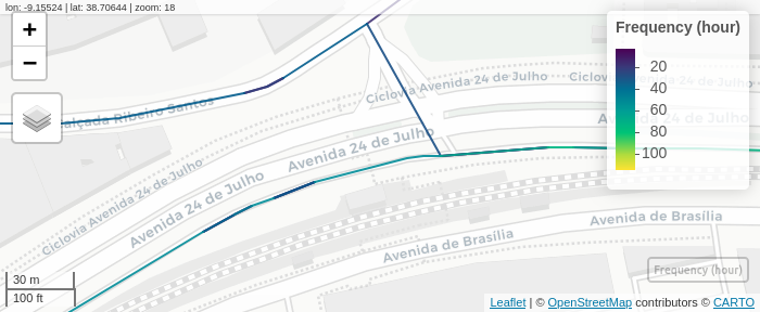
To analyse frequencies at road segments, use
GTFShift::get_way_frequency_hourly(), returning aggregated
results per hour and road segment, using OSM ways.
Mind that routes without an OSM match are ignored. Refer to
GTFShift::osm_shapes_to_routes()for more details.
frequencies_way = GTFShift::get_way_frequency_hourly(gtfs, osm_q)
summary(frequencies_way)
#> way_osm_id hour frequency routes
#> Length :132794 Min. : 0.00 Min. : 1.000 Length :132794
#> N.unique : 6783 1st Qu.: 8.00 1st Qu.: 3.000 N.unique : 3102
#> N.blank : 0 Median :13.00 Median : 6.000 N.blank : 0
#> Min.nchar: 7 Mean :12.56 Mean : 9.654 Min.nchar: 4
#> Max.nchar: 10 3rd Qu.:18.00 3rd Qu.:13.000 Max.nchar: 95
#> Max. :23.00 Max. :99.000
#> geom
#> LINESTRING :132794
#> epsg:4326 : 0
#> +proj=long...: 0
#>
#>
#>
quantile(frequencies_way$frequency)
#> 0% 25% 50% 75% 100%
#> 1 3 6 13 99It returns an sf data.frame that can be
displayed using mapview.
Analyse hourly frequency per route
The frequency analysis can also be performed route wise. For this
purpose, use GTFShift::get_route_frequency_hourly(),
returning aggregated results per hour and route.
The analysis can be performed for each route individually.
By default, the analysis is performed for next business Wednesday, in Portugal. Refer to
GTFShift::calendar_nextBusinessWednesday(), for more details. You can override this, usingdateparameter.
frequencies_route = GTFShift::get_route_frequency_hourly(gtfs)
summary(frequencies_route)
#> route_id route_short_name direction_id hour
#> Length :3359 Length :3359 Min. :0.0000 Min. : 0.00
#> N.unique : 161 N.unique : 111 1st Qu.:0.0000 1st Qu.: 9.00
#> N.blank : 0 N.blank : 0 Median :0.0000 Median :13.00
#> Min.nchar: 4 Min.nchar: 3 Mean :0.4475 Mean :13.15
#> Max.nchar: 5 Max.nchar: 3 3rd Qu.:1.0000 3rd Qu.:18.00
#> Max. :1.0000 Max. :23.00
#> frequency shape_id geom
#> Min. : 1.000 Length :3359 LINESTRING :3359
#> 1st Qu.: 2.000 N.unique : 282 epsg:4326 : 0
#> Median : 3.000 N.blank : 0 +proj=long...: 0
#> Mean : 3.411 Min.nchar: 12
#> 3rd Qu.: 4.000 Max.nchar: 14
#> Max. :12.000
quantile(frequencies_route$frequency)
#> 0% 25% 50% 75% 100%
#> 1 2 3 4 12The overline parameter allows for an even more
aggregated screening of the operation, clustering routes that overlap
and converting them into a single route network. This allows for a
better visualization of the volumes of frequencies per each segment of
the network and can help prioritizing interventions in the network.
frequencies_route_overline = GTFShift::get_route_frequency_hourly(gtfs, overline = TRUE)
summary(frequencies_route_overline)
#> frequency hour geom
#> Min. : 1.00 Min. : 0.00 LINESTRING :138406
#> 1st Qu.: 4.00 1st Qu.: 9.00 epsg:4326 : 0
#> Median : 7.00 Median :13.00 +proj=long...: 0
#> Mean : 10.12 Mean :13.03
#> 3rd Qu.: 13.00 3rd Qu.:18.00
#> Max. :121.00 Max. :23.00
quantile(frequencies_route_overline$frequency)
#> 0% 25% 50% 75% 100%
#> 1 4 7 13 121Improve visualization
Using the overline attribute in
GTFShift::get_route_frequency_hourly() might not be the
best option if the GTFS shapes do not share exactly the same geometry.
In those cases, the overlapping lines might not be merged correctly,
causing inconsistent results, such as a street with different
frequencies along it, despite not having any bus stop in between those
differences.
This is a known issue of
stplanr::overline2(), the method used for the network
aggregation that has not been solved yet.
As an alternative, GTFShift provides some methods that
allow to overcome this issue, by correcting its geometry or aggregating
the network with open data.
Correcting geometry with OSM open data
GTFShift offers several methods that allow to get routes geometry from OpenStreetMaps. Refer to vignette(“osm”) for more details.
Aggregating the network with OSM open data
There are several methods to aggregate a transit network. One approach is through the determination of the centerlines of the roads where the vehicles operate. GTFShift provides a method that encapsulates Python neatnet package for this purpose. Refer to vignette(“osm”) for more details.
During the development of this project, no R packages were found suiting this purpose. Centerline package has this feature in its roadmap. Currently, there are available solutions for Python or ArcGis.
Aggregating frequencies over a target network
As an alternative to the
GTFShift::get_route_frequency_hourly() method using the
overline=TRUE parameter,
GTFShift::network_overline() provides a different frequency
aggregation functionality.
Given a target network, it identifies the segments corresponding to each route and uses them to aggregate the attribute defined in the parameters.
Below is provided an example, that uses the centerlines for the
Carris network as a target network, generated using ArcGis.
GTFShift provides GTFShift::osm_centerlines() method to
generate this kind of network from OSM data. Refer to vignette(“osm”)
for more details.
network = sf::st_read(
"https://github.com/U-Shift/GTFShift/releases/download/v0.5.0/centerline_carris.gpkg",
quiet = TRUE
)
frequencies_route_overline_improved = GTFShift::network_overline(
network,
frequencies_route |> filter(hour == 8),
attr = "frequency"
)
quantile(frequencies_route_overline_improved$frequency)
#> 0% 25% 50% 75% 100%
#> 1 6 11 20 121